numpy.blackman

numpy.blackman(M)

Return the Blackman window.

The Blackman window is a taper formed by using the the first three terms of a summation of cosines. It was designed to have close to the minimal leakage possible. It is close to optimal, only slightly worse than a Kaiser window.

Parameters :

M : int

Number of points in the output window. If zero or less, an empty array is returned.

Returns :

out : ndarray

The window, normalized to one (the value one appears only if the number of samples is odd).

See also

bartlett, hamming, hanning, kaiser

Notes

The Blackman window is defined as

Most references to the Blackman window come from the signal processing literature, where it is used as one of many windowing functions for smoothing values. It is also known as an apodization (which means “removing the foot”, i.e. smoothing discontinuities at the beginning and end of the sampled signal) or tapering function. It is known as a “near optimal” tapering function, almost as good (by some measures) as the kaiser window.

References

Blackman, R.B. and Tukey, J.W., (1958) The measurement of power spectra, Dover Publications, New York.

Oppenheim, A.V., and R.W. Schafer. Discrete-Time Signal Processing. Upper Saddle River, NJ: Prentice-Hall, 1999, pp. 468-471.

Examples

>>> from numpy import blackman
>>> blackman(12)
array([ -1.38777878e-17,   3.26064346e-02,   1.59903635e-01,
         4.14397981e-01,   7.36045180e-01,   9.67046769e-01,
         9.67046769e-01,   7.36045180e-01,   4.14397981e-01,
         1.59903635e-01,   3.26064346e-02,  -1.38777878e-17])

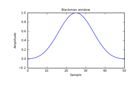
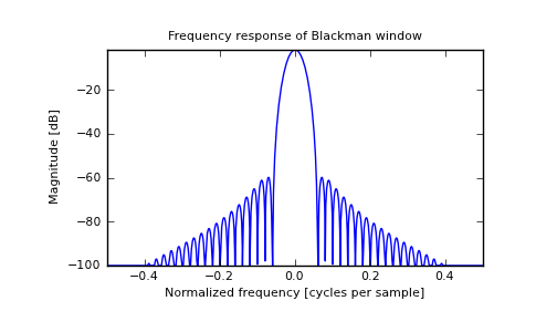
Plot the window and the frequency response:

>>> from numpy import clip, log10, array, blackman, linspace
>>> from numpy.fft import fft, fftshift
>>> import matplotlib.pyplot as plt

>>> window = blackman(51)
>>> plt.plot(window)
[<matplotlib.lines.Line2D object at 0x...>]
>>> plt.title("Blackman window")
<matplotlib.text.Text object at 0x...>
>>> plt.ylabel("Amplitude")
<matplotlib.text.Text object at 0x...>
>>> plt.xlabel("Sample")
<matplotlib.text.Text object at 0x...>
>>> plt.show()

(Source code, png, pdf)

>>> plt.figure()
<matplotlib.figure.Figure object at 0x...>
>>> A = fft(window, 2048) / 25.5
>>> mag = abs(fftshift(A))
>>> freq = linspace(-0.5,0.5,len(A))
>>> response = 20*log10(mag)
>>> response = clip(response,-100,100)
>>> plt.plot(freq, response)
[<matplotlib.lines.Line2D object at 0x...>]
>>> plt.title("Frequency response of Blackman window")
<matplotlib.text.Text object at 0x...>
>>> plt.ylabel("Magnitude [dB]")
<matplotlib.text.Text object at 0x...>
>>> plt.xlabel("Normalized frequency [cycles per sample]")
<matplotlib.text.Text object at 0x...>
>>> plt.axis('tight')
(-0.5, 0.5, -100.0, ...)
>>> plt.show()

(png, pdf)