scipy.stats.shapiro#
- scipy.stats.shapiro(x, *, axis=None, nan_policy='propagate', keepdims=False)[source]#
Perform the Shapiro-Wilk test for normality.
The Shapiro-Wilk test tests the null hypothesis that the data was drawn from a normal distribution.
- Parameters:
- xarray_like
Array of sample data.
- axisint or None, default: None
If an int, the axis of the input along which to compute the statistic. The statistic of each axis-slice (e.g. row) of the input will appear in a corresponding element of the output. If
None, the input will be raveled before computing the statistic.- nan_policy{‘propagate’, ‘omit’, ‘raise’}
Defines how to handle input NaNs.
propagate: if a NaN is present in the axis slice (e.g. row) along which the statistic is computed, the corresponding entry of the output will be NaN.omit: NaNs will be omitted when performing the calculation. If insufficient data remains in the axis slice along which the statistic is computed, the corresponding entry of the output will be NaN.raise: if a NaN is present, aValueErrorwill be raised.
- keepdimsbool, default: False
If this is set to True, the axes which are reduced are left in the result as dimensions with size one. With this option, the result will broadcast correctly against the input array.
- Returns:
- statisticfloat
The test statistic.
- p-valuefloat
The p-value for the hypothesis test.
See also
Notes
The algorithm used is described in [4] but censoring parameters as described are not implemented. For N > 5000 the W test statistic is accurate, but the p-value may not be.
Beginning in SciPy 1.9,
np.matrixinputs (not recommended for new code) are converted tonp.ndarraybefore the calculation is performed. In this case, the output will be a scalar ornp.ndarrayof appropriate shape rather than a 2Dnp.matrix. Similarly, while masked elements of masked arrays are ignored, the output will be a scalar ornp.ndarrayrather than a masked array withmask=False.References
[2] (1,2)Shapiro, S. S. & Wilk, M.B, “An analysis of variance test for normality (complete samples)”, Biometrika, 1965, Vol. 52, pp. 591-611, DOI:10.2307/2333709
[3]Razali, N. M. & Wah, Y. B., “Power comparisons of Shapiro-Wilk, Kolmogorov-Smirnov, Lilliefors and Anderson-Darling tests”, Journal of Statistical Modeling and Analytics, 2011, Vol. 2, pp. 21-33.
[4]Royston P., “Remark AS R94: A Remark on Algorithm AS 181: The W-test for Normality”, 1995, Applied Statistics, Vol. 44, DOI:10.2307/2986146
[5]Phipson B., and Smyth, G. K., “Permutation P-values Should Never Be Zero: Calculating Exact P-values When Permutations Are Randomly Drawn”, Statistical Applications in Genetics and Molecular Biology, 2010, Vol.9, DOI:10.2202/1544-6115.1585
[6]Panagiotakos, D. B., “The value of p-value in biomedical research”, The Open Cardiovascular Medicine Journal, 2008, Vol.2, pp. 97-99, DOI:10.2174/1874192400802010097
Examples
Suppose we wish to infer from measurements whether the weights of adult human males in a medical study are not normally distributed [2]. The weights (lbs) are recorded in the array
xbelow.>>> import numpy as np >>> x = np.array([148, 154, 158, 160, 161, 162, 166, 170, 182, 195, 236])
The normality test of [1] and [2] begins by computing a statistic based on the relationship between the observations and the expected order statistics of a normal distribution.
>>> from scipy import stats
>>> res = stats.shapiro(x)
>>> res.statistic
0.7888147830963135
The value of this statistic tends to be high (close to 1) for samples drawn from a normal distribution.
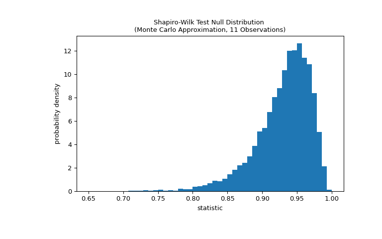
The test is performed by comparing the observed value of the statistic against the null distribution: the distribution of statistic values formed under the null hypothesis that the weights were drawn from a normal distribution. For this normality test, the null distribution is not easy to calculate exactly, so it is usually approximated by Monte Carlo methods, that is, drawing many samples of the same size as
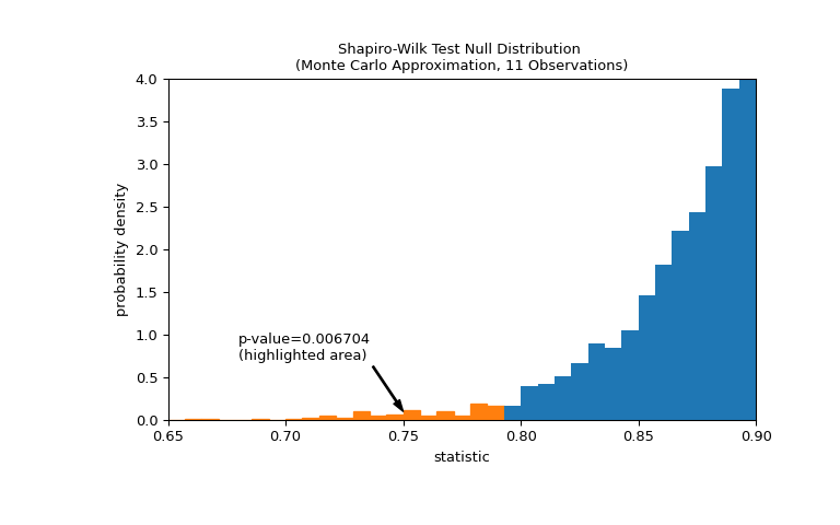
xfrom a normal distribution and computing the values of the statistic for each.>>> def statistic(x): ... # Get only the `shapiro` statistic; ignore its p-value ... return stats.shapiro(x).statistic >>> ref = stats.monte_carlo_test(x, stats.norm.rvs, statistic, ... alternative='less') >>> import matplotlib.pyplot as plt >>> fig, ax = plt.subplots(figsize=(8, 5)) >>> bins = np.linspace(0.65, 1, 50) >>> def plot(ax): # we'll reuse this ... ax.hist(ref.null_distribution, density=True, bins=bins) ... ax.set_title("Shapiro-Wilk Test Null Distribution \n" ... "(Monte Carlo Approximation, 11 Observations)") ... ax.set_xlabel("statistic") ... ax.set_ylabel("probability density") >>> plot(ax) >>> plt.show()
The comparison is quantified by the p-value: the proportion of values in the null distribution less than or equal to the observed value of the statistic.
>>> fig, ax = plt.subplots(figsize=(8, 5))
>>> plot(ax)
>>> annotation = (f'p-value={res.pvalue:.6f}\n(highlighted area)')
>>> props = dict(facecolor='black', width=1, headwidth=5, headlength=8)
>>> _ = ax.annotate(annotation, (0.75, 0.1), (0.68, 0.7), arrowprops=props)
>>> i_extreme = np.where(bins <= res.statistic)[0]
>>> for i in i_extreme:
...     ax.patches[i].set_color('C1')
>>> plt.xlim(0.65, 0.9)
>>> plt.ylim(0, 4)
>>> plt.show
>>> res.pvalue
0.006703833118081093
If the p-value is “small” - that is, if there is a low probability of sampling data from a normally distributed population that produces such an extreme value of the statistic - this may be taken as evidence against the null hypothesis in favor of the alternative: the weights were not drawn from a normal distribution. Note that:
The inverse is not true; that is, the test is not used to provide evidence for the null hypothesis.
The threshold for values that will be considered “small” is a choice that should be made before the data is analyzed [5] with consideration of the risks of both false positives (incorrectly rejecting the null hypothesis) and false negatives (failure to reject a false null hypothesis).