scipy.signal.step2#

scipy.signal.step2(system, X0=None, T=None, N=None, **kwargs)[source]#

Step response of continuous-time system.

This function is functionally the same as scipy.signal.step, but it uses the function scipy.signal.lsim2 to compute the step response.

Parameters

systeman instance of the LTI class or a tuple of array_like

describing the system. The following gives the number of elements in the tuple and the interpretation:

1 (instance of lti)

2 (num, den)

3 (zeros, poles, gain)

4 (A, B, C, D)

X0array_like, optional

Initial state-vector (default is zero).

Tarray_like, optional

Time points (computed if not given).

Nint, optional

Number of time points to compute if T is not given.

kwargsvarious types

Additional keyword arguments are passed on the function scipy.signal.lsim2, which in turn passes them on to scipy.integrate.odeint. See the documentation for scipy.integrate.odeint for information about these arguments.

Returns

T1D ndarray: Output time points.
yout1D ndarray: Step response of system.

See also

scipy.signal.step

Notes

If (num, den) is passed in for system, coefficients for both the numerator and denominator should be specified in descending exponent order (e.g. s^2 + 3s + 5 would be represented as [1, 3, 5]).

New in version 0.8.0.

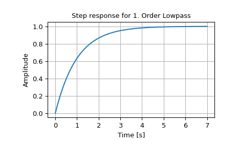
Examples

>>> from scipy import signal
>>> import matplotlib.pyplot as plt
>>> lti = signal.lti([1.0], [1.0, 1.0])
>>> t, y = signal.step2(lti)
>>> plt.plot(t, y)
>>> plt.xlabel('Time [s]')
>>> plt.ylabel('Amplitude')
>>> plt.title('Step response for 1. Order Lowpass')
>>> plt.grid()