scipy.signal.cont2discrete
- scipy.signal.cont2discrete(system, dt, method='zoh', alpha=None)[source]
Transform a continuous to a discrete state-space system.
- Parameters
- systema tuple describing the system or an instance of
lti The following gives the number of elements in the tuple and the interpretation:
1: (instance of
lti)2: (num, den)
3: (zeros, poles, gain)
4: (A, B, C, D)
- dtfloat
The discretization time step.
- methodstr, optional
Which method to use:
gbt: generalized bilinear transformation
bilinear: Tustin’s approximation (“gbt” with alpha=0.5)
euler: Euler (or forward differencing) method (“gbt” with alpha=0)
backward_diff: Backwards differencing (“gbt” with alpha=1.0)
zoh: zero-order hold (default)
foh: first-order hold (versionadded: 1.3.0)
impulse: equivalent impulse response (versionadded: 1.3.0)
- alphafloat within [0, 1], optional
The generalized bilinear transformation weighting parameter, which should only be specified with method=”gbt”, and is ignored otherwise
- systema tuple describing the system or an instance of
- Returns
- sysdtuple containing the discrete system
Based on the input type, the output will be of the form
(num, den, dt) for transfer function input
(zeros, poles, gain, dt) for zeros-poles-gain input
(A, B, C, D, dt) for state-space system input
Notes
By default, the routine uses a Zero-Order Hold (zoh) method to perform the transformation. Alternatively, a generalized bilinear transformation may be used, which includes the common Tustin’s bilinear approximation, an Euler’s method technique, or a backwards differencing technique.
The Zero-Order Hold (zoh) method is based on [1], the generalized bilinear approximation is based on [2] and [3], the First-Order Hold (foh) method is based on [4].
References
- 1
https://en.wikipedia.org/wiki/Discretization#Discretization_of_linear_state_space_models
- 2
http://techteach.no/publications/discretetime_signals_systems/discrete.pdf
- 3
G. Zhang, X. Chen, and T. Chen, Digital redesign via the generalized bilinear transformation, Int. J. Control, vol. 82, no. 4, pp. 741-754, 2009. (https://www.mypolyuweb.hk/~magzhang/Research/ZCC09_IJC.pdf)
- 4
G. F. Franklin, J. D. Powell, and M. L. Workman, Digital control of dynamic systems, 3rd ed. Menlo Park, Calif: Addison-Wesley, pp. 204-206, 1998.
Examples
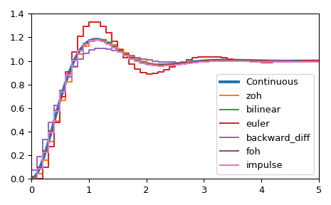
We can transform a continuous state-space system to a discrete one:
>>> import matplotlib.pyplot as plt
>>> from scipy.signal import cont2discrete, lti, dlti, dstep
Define a continuous state-space system.
>>> A = np.array([[0, 1],[-10., -3]])
>>> B = np.array([[0],[10.]])
>>> C = np.array([[1., 0]])
>>> D = np.array([[0.]])
>>> l_system = lti(A, B, C, D)
>>> t, x = l_system.step(T=np.linspace(0, 5, 100))
>>> fig, ax = plt.subplots()
>>> ax.plot(t, x, label='Continuous', linewidth=3)
Transform it to a discrete state-space system using several methods.
>>> dt = 0.1
>>> for method in ['zoh', 'bilinear', 'euler', 'backward_diff', 'foh', 'impulse']:
...    d_system = cont2discrete((A, B, C, D), dt, method=method)
...    s, x_d = dstep(d_system)
...    ax.step(s, np.squeeze(x_d), label=method, where='post')
>>> ax.axis([t[0], t[-1], x[0], 1.4])
>>> ax.legend(loc='best')
>>> fig.tight_layout()
>>> plt.show()
