scipy.special.smirnov
-
scipy.special.smirnov(n, d) = <ufunc 'smirnov'>¶ Kolmogorov-Smirnov complementary cumulative distribution function
Returns the exact Kolmogorov-Smirnov complementary cumulative distribution function,(aka the Survival Function) of Dn+ (or Dn-) for a one-sided test of equality between an empirical and a theoretical distribution. It is equal to the probability that the maximum difference between a theoretical distribution and an empirical one based on n samples is greater than d.
- Parameters
- nint
Number of samples
- dfloat array_like
Deviation between the Empirical CDF (ECDF) and the target CDF.
- Returns
- float
The value(s) of smirnov(n, d), Prob(Dn+ >= d) (Also Prob(Dn- >= d))
See also
smirnoviThe Inverse Survival Function for the distribution
scipy.stats.ksoneProvides the functionality as a continuous distribution
kolmogorov,kolmogiFunctions for the two-sided distribution
Notes
smirnovis used by stats.kstest in the application of the Kolmogorov-Smirnov Goodness of Fit test. For historial reasons this function is exposed in scpy.special, but the recommended way to achieve the most accurate CDF/SF/PDF/PPF/ISF computations is to use the stats.ksone distribution.Examples
>>> from scipy.special import smirnov
Show the probability of a gap at least as big as 0, 0.5 and 1.0 for a sample of size 5
>>> smirnov(5, [0, 0.5, 1.0])
array([ 1.   ,  0.056,  0.   ])
Compare a sample of size 5 drawn from a source N(0.5, 1) distribution against a target N(0, 1) CDF.
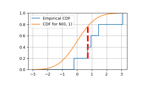
>>> from scipy.stats import norm
>>> n = 5
>>> gendist = norm(0.5, 1)       # Normal distribution, mean 0.5, stddev 1
>>> np.random.seed(seed=233423)  # Set the seed for reproducibility
>>> x = np.sort(gendist.rvs(size=n))
>>> x
array([-0.20946287,  0.71688765,  0.95164151,  1.44590852,  3.08880533])
>>> target = norm(0, 1)
>>> cdfs = target.cdf(x)
>>> cdfs
array([ 0.41704346,  0.76327829,  0.82936059,  0.92589857,  0.99899518])
# Construct the Empirical CDF and the K-S statistics (Dn+, Dn-, Dn)
>>> ecdfs = np.arange(n+1, dtype=float)/n
>>> cols = np.column_stack([x, ecdfs[1:], cdfs, cdfs - ecdfs[:n], ecdfs[1:] - cdfs])
>>> np.set_printoptions(precision=3)
>>> cols
array([[ -2.095e-01,   2.000e-01,   4.170e-01,   4.170e-01,  -2.170e-01],
       [  7.169e-01,   4.000e-01,   7.633e-01,   5.633e-01,  -3.633e-01],
       [  9.516e-01,   6.000e-01,   8.294e-01,   4.294e-01,  -2.294e-01],
       [  1.446e+00,   8.000e-01,   9.259e-01,   3.259e-01,  -1.259e-01],
       [  3.089e+00,   1.000e+00,   9.990e-01,   1.990e-01,   1.005e-03]])
>>> gaps = cols[:, -2:]
>>> Dnpm = np.max(gaps, axis=0)
>>> print('Dn-=%f, Dn+=%f' % (Dnpm[0], Dnpm[1]))
Dn-=0.563278, Dn+=0.001005
>>> probs = smirnov(n, Dnpm)
>>> print(chr(10).join(['For a sample of size %d drawn from a N(0, 1) distribution:' % n,
...      ' Smirnov n=%d: Prob(Dn- >= %f) = %.4f' % (n, Dnpm[0], probs[0]),
...      ' Smirnov n=%d: Prob(Dn+ >= %f) = %.4f' % (n, Dnpm[1], probs[1])]))
For a sample of size 5 drawn from a N(0, 1) distribution:
 Smirnov n=5: Prob(Dn- >= 0.563278) = 0.0250
 Smirnov n=5: Prob(Dn+ >= 0.001005) = 0.9990
Plot the Empirical CDF against the target N(0, 1) CDF
>>> import matplotlib.pyplot as plt
>>> plt.step(np.concatenate([[-3], x]), ecdfs, where='post', label='Empirical CDF')
>>> x3 = np.linspace(-3, 3, 100)
>>> plt.plot(x3, target.cdf(x3), label='CDF for N(0, 1)')
>>> plt.ylim([0, 1]); plt.grid(True); plt.legend();
# Add vertical lines marking Dn+ and Dn-
>>> iminus, iplus = np.argmax(gaps, axis=0)
>>> plt.vlines([x[iminus]], ecdfs[iminus], cdfs[iminus], color='r', linestyle='dashed', lw=4)
>>> plt.vlines([x[iplus]], cdfs[iplus], ecdfs[iplus+1], color='m', linestyle='dashed', lw=4)
>>> plt.show()