scipy.stats.loguniform
-
scipy.stats.loguniform(*args, **kwds) = <scipy.stats._continuous_distns.reciprocal_gen object>[source]¶ A loguniform or reciprocal continuous random variable.
As an instance of the
rv_continuousclass,loguniformobject inherits from it a collection of generic methods (see below for the full list), and completes them with details specific for this particular distribution.Notes
The probability density function for this class is:
\[f(x, a, b) = \frac{1}{x \log(b/a)}\]for \(a \le x \le b\), \(b > a > 0\). This class takes \(a\) and \(b\) as shape parameters.
The probability density above is defined in the “standardized” form. To shift and/or scale the distribution use the
locandscaleparameters. Specifically,loguniform.pdf(x, a, b, loc, scale)is identically equivalent tologuniform.pdf(y, a, b) / scalewithy = (x - loc) / scale. Note that shifting the location of a distribution does not make it a “noncentral” distribution; noncentral generalizations of some distributions are available in separate classes.Examples
>>> from scipy.stats import loguniform
>>> import matplotlib.pyplot as plt
>>> fig, ax = plt.subplots(1, 1)
Calculate a few first moments:
>>> a, b = 0.01, 1
>>> mean, var, skew, kurt = loguniform.stats(a, b, moments='mvsk')
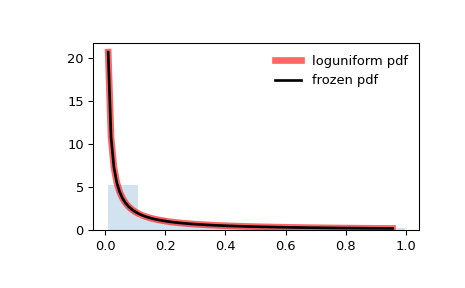
Display the probability density function (
pdf):>>> x = np.linspace(loguniform.ppf(0.01, a, b), ... loguniform.ppf(0.99, a, b), 100) >>> ax.plot(x, loguniform.pdf(x, a, b), ... 'r-', lw=5, alpha=0.6, label='loguniform pdf')
Alternatively, the distribution object can be called (as a function) to fix the shape, location and scale parameters. This returns a “frozen” RV object holding the given parameters fixed.
Freeze the distribution and display the frozen
pdf:>>> rv = loguniform(a, b) >>> ax.plot(x, rv.pdf(x), 'k-', lw=2, label='frozen pdf')
Check accuracy of
cdfandppf:>>> vals = loguniform.ppf([0.001, 0.5, 0.999], a, b) >>> np.allclose([0.001, 0.5, 0.999], loguniform.cdf(vals, a, b)) True
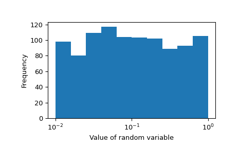
Generate random numbers:
>>> r = loguniform.rvs(a, b, size=1000)
And compare the histogram:
>>> ax.hist(r, density=True, histtype='stepfilled', alpha=0.2)
>>> ax.legend(loc='best', frameon=False)
>>> plt.show()
This doesn’t show the equal probability of
0.01,0.1and1. This is best when the x-axis is log-scaled:>>> import numpy as np >>> fig, ax = plt.subplots(1, 1) >>> ax.hist(np.log10(r)) >>> ax.set_ylabel("Frequency") >>> ax.set_xlabel("Value of random variable") >>> ax.xaxis.set_major_locator(plt.FixedLocator([-2, -1, 0])) >>> ticks = ["$10^{{ {} }}$".format(i) for i in [-2, -1, 0]] >>> ax.set_xticklabels(ticks) >>> plt.show()
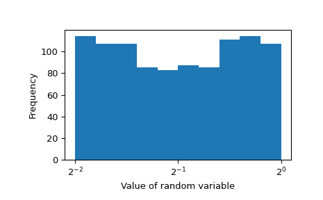
This random variable will be log-uniform regardless of the base chosen for
aandb. Let’s specify with base2instead:>>> rvs = loguniform(2**-2, 2**0).rvs(size=1000)
Values of
1/4,1/2and1are equally likely with this random variable. Here’s the histogram:>>> fig, ax = plt.subplots(1, 1) >>> ax.hist(np.log2(rvs)) >>> ax.set_ylabel("Frequency") >>> ax.set_xlabel("Value of random variable") >>> ax.xaxis.set_major_locator(plt.FixedLocator([-2, -1, 0])) >>> ticks = ["$2^{{ {} }}$".format(i) for i in [-2, -1, 0]] >>> ax.set_xticklabels(ticks) >>> plt.show()
Methods
rvs(a, b, loc=0, scale=1, size=1, random_state=None)
Random variates.
pdf(x, a, b, loc=0, scale=1)
Probability density function.
logpdf(x, a, b, loc=0, scale=1)
Log of the probability density function.
cdf(x, a, b, loc=0, scale=1)
Cumulative distribution function.
logcdf(x, a, b, loc=0, scale=1)
Log of the cumulative distribution function.
sf(x, a, b, loc=0, scale=1)
Survival function (also defined as
1 - cdf, but sf is sometimes more accurate).logsf(x, a, b, loc=0, scale=1)
Log of the survival function.
ppf(q, a, b, loc=0, scale=1)
Percent point function (inverse of
cdf— percentiles).isf(q, a, b, loc=0, scale=1)
Inverse survival function (inverse of
sf).moment(n, a, b, loc=0, scale=1)
Non-central moment of order n
stats(a, b, loc=0, scale=1, moments=’mv’)
Mean(‘m’), variance(‘v’), skew(‘s’), and/or kurtosis(‘k’).
entropy(a, b, loc=0, scale=1)
(Differential) entropy of the RV.
fit(data)
Parameter estimates for generic data. See scipy.stats.rv_continuous.fit for detailed documentation of the keyword arguments.
expect(func, args=(a, b), loc=0, scale=1, lb=None, ub=None, conditional=False, **kwds)
Expected value of a function (of one argument) with respect to the distribution.
median(a, b, loc=0, scale=1)
Median of the distribution.
mean(a, b, loc=0, scale=1)
Mean of the distribution.
var(a, b, loc=0, scale=1)
Variance of the distribution.
std(a, b, loc=0, scale=1)
Standard deviation of the distribution.
interval(alpha, a, b, loc=0, scale=1)
Endpoints of the range that contains alpha percent of the distribution