scipy.interpolate.splprep

scipy.interpolate.splprep(x, w=None, u=None, ub=None, ue=None, k=3, task=0, s=None, t=None, full_output=0, nest=None, per=0, quiet=1)

Find the B-spline representation of an N-D curve.

Given a list of N rank-1 arrays, x, which represent a curve in N-D space parametrized by u, find a smooth approximating spline curve g(u). Uses the FORTRAN routine parcur from FITPACK.

Parameters

xarray_like

A list of sample vector arrays representing the curve.

warray_like, optional

Strictly positive rank-1 array of weights the same length as x[0]. The weights are used in computing the weighted least-squares spline fit. If the errors in the x values have standard-deviation given by the vector d, then w should be 1/d. Default is ones(len(x[0])).

uarray_like, optional

An array of parameter values. If not given, these values are calculated automatically as M = len(x[0]), where

v[0] = 0

v[i] = v[i-1] + distance(x[i], x[i-1])

u[i] = v[i] / v[M-1]

ub, ueint, optional

The end-points of the parameters interval. Defaults to u[0] and u[-1].

kint, optional

Degree of the spline. Cubic splines are recommended. Even values of k should be avoided especially with a small s-value. 1 <= k <= 5, default is 3.

taskint, optional

If task==0 (default), find t and c for a given smoothing factor, s. If task==1, find t and c for another value of the smoothing factor, s. There must have been a previous call with task=0 or task=1 for the same set of data. If task=-1 find the weighted least square spline for a given set of knots, t.

sfloat, optional

A smoothing condition. The amount of smoothness is determined by satisfying the conditions: sum((w * (y - g))**2,axis=0) <= s, where g(x) is the smoothed interpolation of (x,y). The user can use s to control the trade-off between closeness and smoothness of fit. Larger s means more smoothing while smaller values of s indicate less smoothing. Recommended values of s depend on the weights, w. If the weights represent the inverse of the standard-deviation of y, then a good s value should be found in the range (m-sqrt(2*m),m+sqrt(2*m)), where m is the number of data points in x, y, and w.

tint, optional

The knots needed for task=-1.

full_outputint, optional

If non-zero, then return optional outputs.

nestint, optional

An over-estimate of the total number of knots of the spline to help in determining the storage space. By default nest=m/2. Always large enough is nest=m+k+1.

perint, optional

If non-zero, data points are considered periodic with period x[m-1] - x[0] and a smooth periodic spline approximation is returned. Values of y[m-1] and w[m-1] are not used.

quietint, optional

Non-zero to suppress messages. This parameter is deprecated; use standard Python warning filters instead.

Returns

tcktuple

(t,c,k) a tuple containing the vector of knots, the B-spline coefficients, and the degree of the spline.

uarray

An array of the values of the parameter.

fpfloat

The weighted sum of squared residuals of the spline approximation.

ierint

An integer flag about splrep success. Success is indicated if ier<=0. If ier in [1,2,3] an error occurred but was not raised. Otherwise an error is raised.

msgstr

A message corresponding to the integer flag, ier.

See also

splrep, splev, sproot, spalde, splint

bisplrep, bisplev

UnivariateSpline, BivariateSpline

BSpline

make_interp_spline

Notes

See splev for evaluation of the spline and its derivatives. The number of dimensions N must be smaller than 11.

The number of coefficients in the c array is k+1 less then the number of knots, len(t). This is in contrast with splrep, which zero-pads the array of coefficients to have the same length as the array of knots. These additional coefficients are ignored by evaluation routines, splev and BSpline.

References

1

P. Dierckx, “Algorithms for smoothing data with periodic and parametric splines, Computer Graphics and Image Processing”, 20 (1982) 171-184.

2

P. Dierckx, “Algorithms for smoothing data with periodic and parametric splines”, report tw55, Dept. Computer Science, K.U.Leuven, 1981.

3

P. Dierckx, “Curve and surface fitting with splines”, Monographs on Numerical Analysis, Oxford University Press, 1993.

Examples

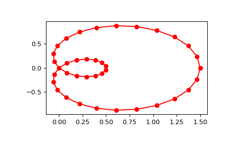
Generate a discretization of a limacon curve in the polar coordinates:

>>> phi = np.linspace(0, 2.*np.pi, 40)
>>> r = 0.5 + np.cos(phi)         # polar coords
>>> x, y = r * np.cos(phi), r * np.sin(phi)    # convert to cartesian

And interpolate:

>>> from scipy.interpolate import splprep, splev
>>> tck, u = splprep([x, y], s=0)
>>> new_points = splev(u, tck)

Notice that (i) we force interpolation by using s=0, (ii) the parameterization, u, is generated automatically. Now plot the result:

>>> import matplotlib.pyplot as plt
>>> fig, ax = plt.subplots()
>>> ax.plot(x, y, 'ro')
>>> ax.plot(new_points[0], new_points[1], 'r-')
>>> plt.show()