Spatial data structures and algorithms (scipy.spatial)
scipy.spatial can compute triangulations, Voronoi diagrams, and
convex hulls of a set of points, by leveraging the Qhull library.
Moreover, it contains KDTree implementations for nearest-neighbor point
queries, and utilities for distance computations in various metrics.
Delaunay triangulations
The Delaunay triangulation is a subdivision of a set of points into a non-overlapping set of triangles, such that no point is inside the circumcircle of any triangle. In practice, such triangulations tend to avoid triangles with small angles.
Delaunay triangulation can be computed using scipy.spatial as follows:
>>> from scipy.spatial import Delaunay
>>> points = np.array([[0, 0], [0, 1.1], [1, 0], [1, 1]])
>>> tri = Delaunay(points)
We can visualize it:
>>> import matplotlib.pyplot as plt
>>> plt.triplot(points[:,0], points[:,1], tri.simplices)
>>> plt.plot(points[:,0], points[:,1], 'o')
And add some further decorations:
>>> for j, p in enumerate(points):
...     plt.text(p[0]-0.03, p[1]+0.03, j, ha='right') # label the points
>>> for j, s in enumerate(tri.simplices):
...     p = points[s].mean(axis=0)
...     plt.text(p[0], p[1], '#%d' % j, ha='center') # label triangles
>>> plt.xlim(-0.5, 1.5); plt.ylim(-0.5, 1.5)
>>> plt.show()
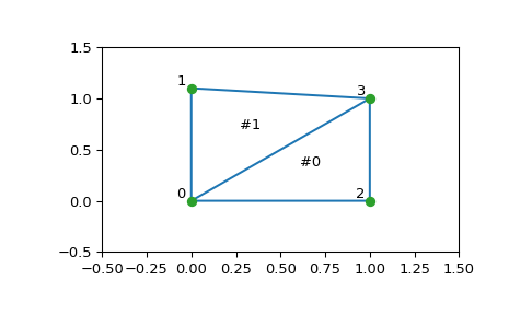
The structure of the triangulation is encoded in the following way:
the simplices attribute contains the indices of the points in the
points array that make up the triangle. For instance:
>>> i = 1
>>> tri.simplices[i,:]
array([3, 1, 0], dtype=int32)
>>> points[tri.simplices[i,:]]
array([[ 1. ,  1. ],
       [ 0. ,  1.1],
       [ 0. ,  0. ]])
Moreover, neighboring triangles can also be found:
>>> tri.neighbors[i]
array([-1,  0, -1], dtype=int32)
What this tells us is that this triangle has triangle #0 as a neighbor, but no other neighbors. Moreover, it tells us that neighbor 0 is opposite the vertex 1 of the triangle:
>>> points[tri.simplices[i, 1]]
array([ 0. ,  1.1])
Indeed, from the figure, we see that this is the case.
Qhull can also perform tessellations to simplices for higher-dimensional point sets (for instance, subdivision into tetrahedra in 3-D).
Coplanar points
It is important to note that not all points necessarily appear as vertices of the triangulation, due to numerical precision issues in forming the triangulation. Consider the above with a duplicated point:
>>> points = np.array([[0, 0], [0, 1], [1, 0], [1, 1], [1, 1]])
>>> tri = Delaunay(points)
>>> np.unique(tri.simplices.ravel())
array([0, 1, 2, 3], dtype=int32)
Observe that point #4, which is a duplicate, does not occur as a vertex of the triangulation. That this happened is recorded:
>>> tri.coplanar
array([[4, 0, 3]], dtype=int32)
This means that point 4 resides near triangle 0 and vertex 3, but is not included in the triangulation.
Note that such degeneracies can occur not only because of duplicated points, but also for more complicated geometrical reasons, even in point sets that at first sight seem well-behaved.
However, Qhull has the “QJ” option, which instructs it to perturb the input data randomly until degeneracies are resolved:
>>> tri = Delaunay(points, qhull_options="QJ Pp")
>>> points[tri.simplices]
array([[[1, 0],
        [1, 1],
        [0, 0]],
       [[1, 1],
        [1, 1],
        [1, 0]],
       [[1, 1],
        [0, 1],
        [0, 0]],
       [[0, 1],
        [1, 1],
        [1, 1]]])
Two new triangles appeared. However, we see that they are degenerate and have zero area.
Convex hulls
A convex hull is the smallest convex object containing all points in a given point set.
These can be computed via the Qhull wrappers in scipy.spatial as
follows:
>>> from scipy.spatial import ConvexHull
>>> points = np.random.rand(30, 2)   # 30 random points in 2-D
>>> hull = ConvexHull(points)
The convex hull is represented as a set of N 1-D simplices, which in 2-D means line segments. The storage scheme is exactly the same as for the simplices in the Delaunay triangulation discussed above.
We can illustrate the above result:
>>> import matplotlib.pyplot as plt
>>> plt.plot(points[:,0], points[:,1], 'o')
>>> for simplex in hull.simplices:
...     plt.plot(points[simplex,0], points[simplex,1], 'k-')
>>> plt.show()
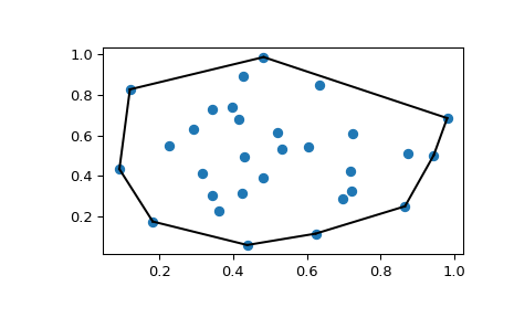
The same can be achieved with scipy.spatial.convex_hull_plot_2d.
Voronoi diagrams
A Voronoi diagram is a subdivision of the space into the nearest neighborhoods of a given set of points.
There are two ways to approach this object using scipy.spatial.
First, one can use the KDTree to answer the question “which of the
points is closest to this one”, and define the regions that way:
>>> from scipy.spatial import KDTree
>>> points = np.array([[0, 0], [0, 1], [0, 2], [1, 0], [1, 1], [1, 2],
...                    [2, 0], [2, 1], [2, 2]])
>>> tree = KDTree(points)
>>> tree.query([0.1, 0.1])
(0.14142135623730953, 0)
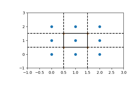
So the point (0.1, 0.1) belongs to region 0. In color:
>>> x = np.linspace(-0.5, 2.5, 31)
>>> y = np.linspace(-0.5, 2.5, 33)
>>> xx, yy = np.meshgrid(x, y)
>>> xy = np.c_[xx.ravel(), yy.ravel()]
>>> import matplotlib.pyplot as plt
>>> dx_half, dy_half = np.diff(x[:2])[0] / 2., np.diff(y[:2])[0] / 2.
>>> x_edges = np.concatenate((x - dx_half, [x[-1] + dx_half]))
>>> y_edges = np.concatenate((y - dy_half, [y[-1] + dy_half]))
>>> plt.pcolormesh(x_edges, y_edges, tree.query(xy)[1].reshape(33, 31), shading='flat')
>>> plt.plot(points[:,0], points[:,1], 'ko')
>>> plt.show()
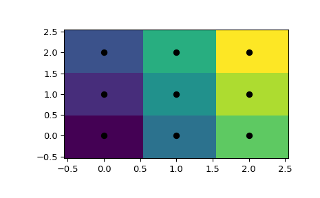
This does not, however, give the Voronoi diagram as a geometrical object.
The representation in terms of lines and points can be again
obtained via the Qhull wrappers in scipy.spatial:
>>> from scipy.spatial import Voronoi
>>> vor = Voronoi(points)
>>> vor.vertices
array([[0.5, 0.5],
       [0.5, 1.5],
       [1.5, 0.5],
       [1.5, 1.5]])
The Voronoi vertices denote the set of points forming the polygonal edges of the Voronoi regions. In this case, there are 9 different regions:
>>> vor.regions
[[], [-1, 0], [-1, 1], [1, -1, 0], [3, -1, 2], [-1, 3], [-1, 2], [0, 1, 3, 2], [2, -1, 0], [3, -1, 1]]
Negative value -1 again indicates a point at infinity. Indeed,
only one of the regions, [0, 1, 3, 2], is bounded. Note here that
due to similar numerical precision issues as in Delaunay triangulation
above, there may be fewer Voronoi regions than input points.
The ridges (lines in 2-D) separating the regions are described as a similar collection of simplices as the convex hull pieces:
>>> vor.ridge_vertices
[[-1, 0], [-1, 0], [-1, 1], [-1, 1], [0, 1], [-1, 3], [-1, 2], [2, 3], [-1, 3], [-1, 2], [1, 3], [0, 2]]
These numbers present the indices of the Voronoi vertices making up the
line segments. -1 is again a point at infinity — only 4 of
the 12 lines are a bounded line segment, while others extend to
infinity.
The Voronoi ridges are perpendicular to the lines drawn between the input points. To which two points each ridge corresponds is also recorded:
>>> vor.ridge_points
array([[0, 3],
       [0, 1],
       [2, 5],
       [2, 1],
       [1, 4],
       [7, 8],
       [7, 6],
       [7, 4],
       [8, 5],
       [6, 3],
       [4, 5],
       [4, 3]], dtype=int32)
This information, taken together, is enough to construct the full diagram.
We can plot it as follows. First, the points and the Voronoi vertices:
>>> plt.plot(points[:, 0], points[:, 1], 'o')
>>> plt.plot(vor.vertices[:, 0], vor.vertices[:, 1], '*')
>>> plt.xlim(-1, 3); plt.ylim(-1, 3)
Plotting the finite line segments goes as for the convex hull, but now we have to guard for the infinite edges:
>>> for simplex in vor.ridge_vertices:
...     simplex = np.asarray(simplex)
...     if np.all(simplex >= 0):
...         plt.plot(vor.vertices[simplex, 0], vor.vertices[simplex, 1], 'k-')
The ridges extending to infinity require a bit more care:
>>> center = points.mean(axis=0)
>>> for pointidx, simplex in zip(vor.ridge_points, vor.ridge_vertices):
...     simplex = np.asarray(simplex)
...     if np.any(simplex < 0):
...         i = simplex[simplex >= 0][0] # finite end Voronoi vertex
...         t = points[pointidx[1]] - points[pointidx[0]]  # tangent
...         t = t / np.linalg.norm(t)
...         n = np.array([-t[1], t[0]]) # normal
...         midpoint = points[pointidx].mean(axis=0)
...         far_point = vor.vertices[i] + np.sign(np.dot(midpoint - center, n)) * n * 100
...         plt.plot([vor.vertices[i,0], far_point[0]],
...                  [vor.vertices[i,1], far_point[1]], 'k--')
>>> plt.show()
This plot can also be created using scipy.spatial.voronoi_plot_2d.
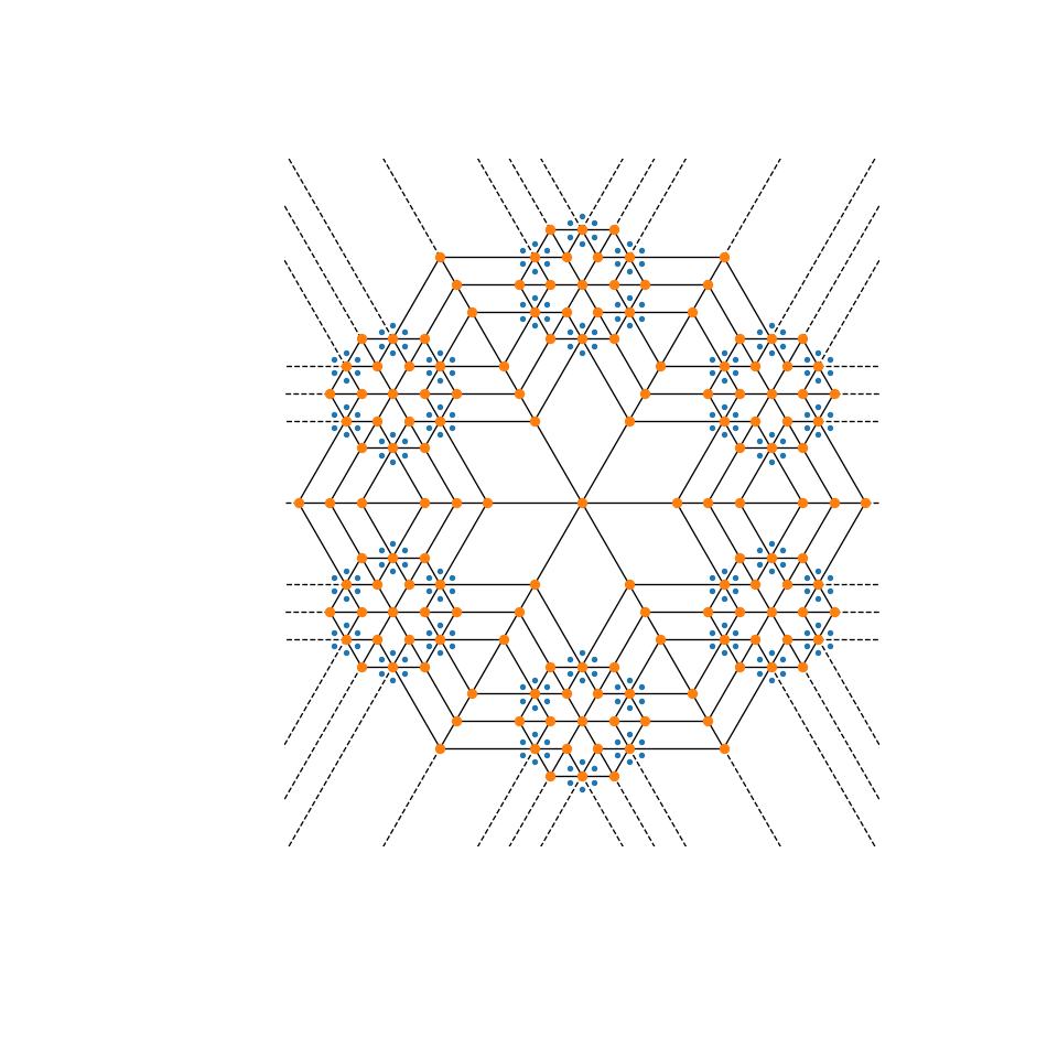
Voronoi diagrams can be used to create interesting generative art. Try playing
with the settings of this mandala function to create your own!
>>> import numpy as np
>>> from scipy import spatial
>>> import matplotlib.pyplot as plt
>>> def mandala(n_iter, n_points, radius):
...     """Creates a mandala figure using Voronoi tesselations.
...
...     Parameters
...     ----------
...     n_iter : int
...         Number of iterations, i.e. how many times the equidistant points will
...         be generated.
...     n_points : int
...         Number of points to draw per iteration.
...     radius : scalar
...         The radial expansion factor.
...
...     Returns
...     -------
...     fig : matplotlib.Figure instance
...
...     Notes
...     -----
...     This code is adapted from the work of Audrey Roy Greenfeld [1]_ and Carlos
...     Focil-Espinosa [2]_, who created beautiful mandalas with Python code.  That
...     code in turn was based on Antonio Sánchez Chinchón's R code [3]_.
...
...     References
...     ----------
...     .. [1] https://www.codemakesmehappy.com/2019/09/voronoi-mandalas.html
...
...     .. [2] https://github.com/CarlosFocil/mandalapy
...
...     .. [3] https://github.com/aschinchon/mandalas
...
...     """
...     fig = plt.figure(figsize=(10, 10))
...     ax = fig.add_subplot(111)
...     ax.set_axis_off()
...     ax.set_aspect('equal', adjustable='box')
...
...     angles = np.linspace(0, 2*np.pi * (1 - 1/n_points), num=n_points) + np.pi/2
...     # Starting from a single center point, add points iteratively
...     xy = np.array([[0, 0]])
...     for k in range(n_iter):
...         t1 = np.array([])
...         t2 = np.array([])
...         # Add `n_points` new points around each existing point in this iteration
...         for i in range(xy.shape[0]):
...             t1 = np.append(t1, xy[i, 0] + radius**k * np.cos(angles))
...             t2 = np.append(t2, xy[i, 1] + radius**k * np.sin(angles))
...
...         xy = np.column_stack((t1, t2))
...
...     # Create the Mandala figure via a Voronoi plot
...     spatial.voronoi_plot_2d(spatial.Voronoi(xy), ax=ax)
...
...     return fig
>>> # Modify the following parameters in order to get different figures
>>> n_iter = 3
>>> n_points = 6
>>> radius = 4
>>> fig = mandala(n_iter, n_points, radius)
>>> plt.show()