scipy.signal.windows.slepian
-
scipy.signal.windows.slepian(M, width, sym=True)[source]¶ Return a digital Slepian (DPSS) window.
Used to maximize the energy concentration in the main lobe. Also called the digital prolate spheroidal sequence (DPSS).
Note
Deprecated in SciPy 1.1.
slepianwill be removed in a future version of SciPy, it is replaced bydpss, which uses the standard definition of a digital Slepian window.- Parameters
- Mint
Number of points in the output window. If zero or less, an empty array is returned.
- widthfloat
Bandwidth
- symbool, optional
When True (default), generates a symmetric window, for use in filter design. When False, generates a periodic window, for use in spectral analysis.
- Returns
- wndarray
The window, with the maximum value always normalized to 1
See also
References
- 1
D. Slepian & H. O. Pollak: “Prolate spheroidal wave functions, Fourier analysis and uncertainty-I,” Bell Syst. Tech. J., vol.40, pp.43-63, 1961. https://archive.org/details/bstj40-1-43
- 2
H. J. Landau & H. O. Pollak: “Prolate spheroidal wave functions, Fourier analysis and uncertainty-II,” Bell Syst. Tech. J. , vol.40, pp.65-83, 1961. https://archive.org/details/bstj40-1-65
Examples
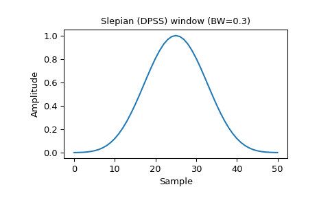
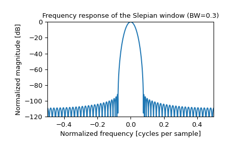
Plot the window and its frequency response:
>>> from scipy import signal
>>> from scipy.fft import fft, fftshift
>>> import matplotlib.pyplot as plt
>>> window = signal.slepian(51, width=0.3)
>>> plt.plot(window)
>>> plt.title("Slepian (DPSS) window (BW=0.3)")
>>> plt.ylabel("Amplitude")
>>> plt.xlabel("Sample")
>>> plt.figure()
>>> A = fft(window, 2048) / (len(window)/2.0)
>>> freq = np.linspace(-0.5, 0.5, len(A))
>>> response = 20 * np.log10(np.abs(fftshift(A / abs(A).max())))
>>> plt.plot(freq, response)
>>> plt.axis([-0.5, 0.5, -120, 0])
>>> plt.title("Frequency response of the Slepian window (BW=0.3)")
>>> plt.ylabel("Normalized magnitude [dB]")
>>> plt.xlabel("Normalized frequency [cycles per sample]")