scipy.integrate.solve_ivp
-
scipy.integrate.solve_ivp(fun, t_span, y0, method='RK45', t_eval=None, dense_output=False, events=None, vectorized=False, args=None, **options)[source]¶ Solve an initial value problem for a system of ODEs.
This function numerically integrates a system of ordinary differential equations given an initial value:
dy / dt = f(t, y)
y(t0) = y0
Here t is a 1-D independent variable (time), y(t) is an N-D vector-valued function (state), and an N-D vector-valued function f(t, y) determines the differential equations. The goal is to find y(t) approximately satisfying the differential equations, given an initial value y(t0)=y0.
Some of the solvers support integration in the complex domain, but note that for stiff ODE solvers, the right-hand side must be complex-differentiable (satisfy Cauchy-Riemann equations [11]). To solve a problem in the complex domain, pass y0 with a complex data type. Another option always available is to rewrite your problem for real and imaginary parts separately.
- Parameters
- funcallable
Right-hand side of the system. The calling signature is
fun(t, y). Here t is a scalar, and there are two options for the ndarray y: It can either have shape (n,); then fun must return array_like with shape (n,). Alternatively, it can have shape (n, k); then fun must return an array_like with shape (n, k), i.e., each column corresponds to a single column in y. The choice between the two options is determined by vectorized argument (see below). The vectorized implementation allows a faster approximation of the Jacobian by finite differences (required for stiff solvers).- t_span2-tuple of floats
Interval of integration (t0, tf). The solver starts with t=t0 and integrates until it reaches t=tf.
- y0array_like, shape (n,)
Initial state. For problems in the complex domain, pass y0 with a complex data type (even if the initial value is purely real).
- methodstring or
OdeSolver, optional Integration method to use:
‘RK45’ (default): Explicit Runge-Kutta method of order 5(4) [1]. The error is controlled assuming accuracy of the fourth-order method, but steps are taken using the fifth-order accurate formula (local extrapolation is done). A quartic interpolation polynomial is used for the dense output [2]. Can be applied in the complex domain.
‘RK23’: Explicit Runge-Kutta method of order 3(2) [3]. The error is controlled assuming accuracy of the second-order method, but steps are taken using the third-order accurate formula (local extrapolation is done). A cubic Hermite polynomial is used for the dense output. Can be applied in the complex domain.
‘DOP853’: Explicit Runge-Kutta method of order 8 [13]. Python implementation of the “DOP853” algorithm originally written in Fortran [14]. A 7-th order interpolation polynomial accurate to 7-th order is used for the dense output. Can be applied in the complex domain.
‘Radau’: Implicit Runge-Kutta method of the Radau IIA family of order 5 [4]. The error is controlled with a third-order accurate embedded formula. A cubic polynomial which satisfies the collocation conditions is used for the dense output.
‘BDF’: Implicit multi-step variable-order (1 to 5) method based on a backward differentiation formula for the derivative approximation [5]. The implementation follows the one described in [6]. A quasi-constant step scheme is used and accuracy is enhanced using the NDF modification. Can be applied in the complex domain.
‘LSODA’: Adams/BDF method with automatic stiffness detection and switching [7], [8]. This is a wrapper of the Fortran solver from ODEPACK.
Explicit Runge-Kutta methods (‘RK23’, ‘RK45’, ‘DOP853’) should be used for non-stiff problems and implicit methods (‘Radau’, ‘BDF’) for stiff problems [9]. Among Runge-Kutta methods, ‘DOP853’ is recommended for solving with high precision (low values of rtol and atol).
If not sure, first try to run ‘RK45’. If it makes unusually many iterations, diverges, or fails, your problem is likely to be stiff and you should use ‘Radau’ or ‘BDF’. ‘LSODA’ can also be a good universal choice, but it might be somewhat less convenient to work with as it wraps old Fortran code.
You can also pass an arbitrary class derived from
OdeSolverwhich implements the solver.- t_evalarray_like or None, optional
Times at which to store the computed solution, must be sorted and lie within t_span. If None (default), use points selected by the solver.
- dense_outputbool, optional
Whether to compute a continuous solution. Default is False.
- eventscallable, or list of callables, optional
Events to track. If None (default), no events will be tracked. Each event occurs at the zeros of a continuous function of time and state. Each function must have the signature
event(t, y)and return a float. The solver will find an accurate value of t at whichevent(t, y(t)) = 0using a root-finding algorithm. By default, all zeros will be found. The solver looks for a sign change over each step, so if multiple zero crossings occur within one step, events may be missed. Additionally each event function might have the following attributes:- terminal: bool, optional
Whether to terminate integration if this event occurs. Implicitly False if not assigned.
- direction: float, optional
Direction of a zero crossing. If direction is positive, event will only trigger when going from negative to positive, and vice versa if direction is negative. If 0, then either direction will trigger event. Implicitly 0 if not assigned.
You can assign attributes like
event.terminal = Trueto any function in Python.- vectorizedbool, optional
Whether fun is implemented in a vectorized fashion. Default is False.
- argstuple, optional
Additional arguments to pass to the user-defined functions. If given, the additional arguments are passed to all user-defined functions. So if, for example, fun has the signature
fun(t, y, a, b, c), then jac (if given) and any event functions must have the same signature, and args must be a tuple of length 3.- options
Options passed to a chosen solver. All options available for already implemented solvers are listed below.
- first_stepfloat or None, optional
Initial step size. Default is None which means that the algorithm should choose.
- max_stepfloat, optional
Maximum allowed step size. Default is np.inf, i.e., the step size is not bounded and determined solely by the solver.
- rtol, atolfloat or array_like, optional
Relative and absolute tolerances. The solver keeps the local error estimates less than
atol + rtol * abs(y). Here rtol controls a relative accuracy (number of correct digits). But if a component of y is approximately below atol, the error only needs to fall within the same atol threshold, and the number of correct digits is not guaranteed. If components of y have different scales, it might be beneficial to set different atol values for different components by passing array_like with shape (n,) for atol. Default values are 1e-3 for rtol and 1e-6 for atol.- jacarray_like, sparse_matrix, callable or None, optional
Jacobian matrix of the right-hand side of the system with respect to y, required by the ‘Radau’, ‘BDF’ and ‘LSODA’ method. The Jacobian matrix has shape (n, n) and its element (i, j) is equal to
d f_i / d y_j. There are three ways to define the Jacobian:If array_like or sparse_matrix, the Jacobian is assumed to be constant. Not supported by ‘LSODA’.
If callable, the Jacobian is assumed to depend on both t and y; it will be called as
jac(t, y), as necessary. For ‘Radau’ and ‘BDF’ methods, the return value might be a sparse matrix.If None (default), the Jacobian will be approximated by finite differences.
It is generally recommended to provide the Jacobian rather than relying on a finite-difference approximation.
- jac_sparsityarray_like, sparse matrix or None, optional
Defines a sparsity structure of the Jacobian matrix for a finite- difference approximation. Its shape must be (n, n). This argument is ignored if jac is not None. If the Jacobian has only few non-zero elements in each row, providing the sparsity structure will greatly speed up the computations [10]. A zero entry means that a corresponding element in the Jacobian is always zero. If None (default), the Jacobian is assumed to be dense. Not supported by ‘LSODA’, see lband and uband instead.
- lband, ubandint or None, optional
Parameters defining the bandwidth of the Jacobian for the ‘LSODA’ method, i.e.,
jac[i, j] != 0 only for i - lband <= j <= i + uband. Default is None. Setting these requires your jac routine to return the Jacobian in the packed format: the returned array must havencolumns anduband + lband + 1rows in which Jacobian diagonals are written. Specificallyjac_packed[uband + i - j , j] = jac[i, j]. The same format is used inscipy.linalg.solve_banded(check for an illustration). These parameters can be also used withjac=Noneto reduce the number of Jacobian elements estimated by finite differences.- min_stepfloat, optional
The minimum allowed step size for ‘LSODA’ method. By default min_step is zero.
- Returns
- Bunch object with the following fields defined:
- tndarray, shape (n_points,)
Time points.
- yndarray, shape (n, n_points)
Values of the solution at t.
- sol
OdeSolutionor None Found solution as
OdeSolutioninstance; None if dense_output was set to False.- t_eventslist of ndarray or None
Contains for each event type a list of arrays at which an event of that type event was detected. None if events was None.
- y_eventslist of ndarray or None
For each value of t_events, the corresponding value of the solution. None if events was None.
- nfevint
Number of evaluations of the right-hand side.
- njevint
Number of evaluations of the Jacobian.
- nluint
Number of LU decompositions.
- statusint
Reason for algorithm termination:
-1: Integration step failed.
0: The solver successfully reached the end of tspan.
1: A termination event occurred.
- messagestring
Human-readable description of the termination reason.
- successbool
True if the solver reached the interval end or a termination event occurred (
status >= 0).
References
- 1
J. R. Dormand, P. J. Prince, “A family of embedded Runge-Kutta formulae”, Journal of Computational and Applied Mathematics, Vol. 6, No. 1, pp. 19-26, 1980.
- 2
L. W. Shampine, “Some Practical Runge-Kutta Formulas”, Mathematics of Computation,, Vol. 46, No. 173, pp. 135-150, 1986.
- 3
P. Bogacki, L.F. Shampine, “A 3(2) Pair of Runge-Kutta Formulas”, Appl. Math. Lett. Vol. 2, No. 4. pp. 321-325, 1989.
- 4
E. Hairer, G. Wanner, “Solving Ordinary Differential Equations II: Stiff and Differential-Algebraic Problems”, Sec. IV.8.
- 5
Backward Differentiation Formula on Wikipedia.
- 6
L. F. Shampine, M. W. Reichelt, “THE MATLAB ODE SUITE”, SIAM J. SCI. COMPUTE., Vol. 18, No. 1, pp. 1-22, January 1997.
- 7
A. C. Hindmarsh, “ODEPACK, A Systematized Collection of ODE Solvers,” IMACS Transactions on Scientific Computation, Vol 1., pp. 55-64, 1983.
- 8
L. Petzold, “Automatic selection of methods for solving stiff and nonstiff systems of ordinary differential equations”, SIAM Journal on Scientific and Statistical Computing, Vol. 4, No. 1, pp. 136-148, 1983.
- 9
Stiff equation on Wikipedia.
- 10
A. Curtis, M. J. D. Powell, and J. Reid, “On the estimation of sparse Jacobian matrices”, Journal of the Institute of Mathematics and its Applications, 13, pp. 117-120, 1974.
- 11
Cauchy-Riemann equations on Wikipedia.
- 12
Lotka-Volterra equations on Wikipedia.
- 13
E. Hairer, S. P. Norsett G. Wanner, “Solving Ordinary Differential Equations I: Nonstiff Problems”, Sec. II.
- 14
Examples
Basic exponential decay showing automatically chosen time points.
>>> from scipy.integrate import solve_ivp
>>> def exponential_decay(t, y): return -0.5 * y
>>> sol = solve_ivp(exponential_decay, [0, 10], [2, 4, 8])
>>> print(sol.t)
[ 0.          0.11487653  1.26364188  3.06061781  4.81611105  6.57445806
  8.33328988 10.        ]
>>> print(sol.y)
[[2.         1.88836035 1.06327177 0.43319312 0.18017253 0.07483045
  0.03107158 0.01350781]
 [4.         3.7767207  2.12654355 0.86638624 0.36034507 0.14966091
  0.06214316 0.02701561]
 [8.         7.5534414  4.25308709 1.73277247 0.72069014 0.29932181
  0.12428631 0.05403123]]
Specifying points where the solution is desired.
>>> sol = solve_ivp(exponential_decay, [0, 10], [2, 4, 8],
...                 t_eval=[0, 1, 2, 4, 10])
>>> print(sol.t)
[ 0  1  2  4 10]
>>> print(sol.y)
[[2.         1.21305369 0.73534021 0.27066736 0.01350938]
 [4.         2.42610739 1.47068043 0.54133472 0.02701876]
 [8.         4.85221478 2.94136085 1.08266944 0.05403753]]
Cannon fired upward with terminal event upon impact. The
terminalanddirectionfields of an event are applied by monkey patching a function. Herey[0]is position andy[1]is velocity. The projectile starts at position 0 with velocity +10. Note that the integration never reaches t=100 because the event is terminal.>>> def upward_cannon(t, y): return [y[1], -0.5] >>> def hit_ground(t, y): return y[0] >>> hit_ground.terminal = True >>> hit_ground.direction = -1 >>> sol = solve_ivp(upward_cannon, [0, 100], [0, 10], events=hit_ground) >>> print(sol.t_events) [array([40.])] >>> print(sol.t) [0.00000000e+00 9.99900010e-05 1.09989001e-03 1.10988901e-02 1.11088891e-01 1.11098890e+00 1.11099890e+01 4.00000000e+01]
Use dense_output and events to find position, which is 100, at the apex of the cannonball’s trajectory. Apex is not defined as terminal, so both apex and hit_ground are found. There is no information at t=20, so the sol attribute is used to evaluate the solution. The sol attribute is returned by setting
dense_output=True. Alternatively, the y_events attribute can be used to access the solution at the time of the event.>>> def apex(t, y): return y[1] >>> sol = solve_ivp(upward_cannon, [0, 100], [0, 10], ... events=(hit_ground, apex), dense_output=True) >>> print(sol.t_events) [array([40.]), array([20.])] >>> print(sol.t) [0.00000000e+00 9.99900010e-05 1.09989001e-03 1.10988901e-02 1.11088891e-01 1.11098890e+00 1.11099890e+01 4.00000000e+01] >>> print(sol.sol(sol.t_events[1][0])) [100. 0.] >>> print(sol.y_events) [array([[-5.68434189e-14, -1.00000000e+01]]), array([[1.00000000e+02, 1.77635684e-15]])]
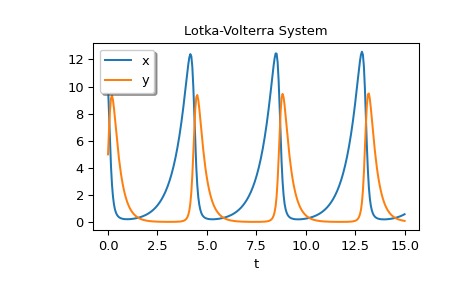
As an example of a system with additional parameters, we’ll implement the Lotka-Volterra equations [12].
>>> def lotkavolterra(t, z, a, b, c, d):
...     x, y = z
...     return [a*x - b*x*y, -c*y + d*x*y]
...
We pass in the parameter values a=1.5, b=1, c=3 and d=1 with the args argument.
>>> sol = solve_ivp(lotkavolterra, [0, 15], [10, 5], args=(1.5, 1, 3, 1),
...                 dense_output=True)
Compute a dense solution and plot it.
>>> t = np.linspace(0, 15, 300)
>>> z = sol.sol(t)
>>> import matplotlib.pyplot as plt
>>> plt.plot(t, z.T)
>>> plt.xlabel('t')
>>> plt.legend(['x', 'y'], shadow=True)
>>> plt.title('Lotka-Volterra System')
>>> plt.show()