Optimization (scipy.optimize)
Contents
-
Unconstrained minimization of multivariate scalar functions (
minimize)Constrained minimization of multivariate scalar functions (
minimize)
The scipy.optimize package provides several commonly used
optimization algorithms. A detailed listing is available:
scipy.optimize (can also be found by help(scipy.optimize)).
Unconstrained minimization of multivariate scalar functions (minimize)
The minimize function provides a common interface to unconstrained
and constrained minimization algorithms for multivariate scalar functions
in scipy.optimize. To demonstrate the minimization function, consider the
problem of minimizing the Rosenbrock function of \(N\) variables:
The minimum value of this function is 0 which is achieved when \(x_{i}=1.\)
Note that the Rosenbrock function and its derivatives are included in
scipy.optimize. The implementations shown in the following sections
provide examples of how to define an objective function as well as its
jacobian and hessian functions.
Nelder-Mead Simplex algorithm (method='Nelder-Mead')
In the example below, the minimize routine is used
with the Nelder-Mead simplex algorithm (selected through the method
parameter):
>>> import numpy as np
>>> from scipy.optimize import minimize
>>> def rosen(x):
...     """The Rosenbrock function"""
...     return sum(100.0*(x[1:]-x[:-1]**2.0)**2.0 + (1-x[:-1])**2.0)
>>> x0 = np.array([1.3, 0.7, 0.8, 1.9, 1.2])
>>> res = minimize(rosen, x0, method='nelder-mead',
...                options={'xatol': 1e-8, 'disp': True})
Optimization terminated successfully.
         Current function value: 0.000000
         Iterations: 339
         Function evaluations: 571
>>> print(res.x)
[1. 1. 1. 1. 1.]
The simplex algorithm is probably the simplest way to minimize a fairly well-behaved function. It requires only function evaluations and is a good choice for simple minimization problems. However, because it does not use any gradient evaluations, it may take longer to find the minimum.
Another optimization algorithm that needs only function calls to find
the minimum is Powell’s method available by setting method='powell' in
minimize.
Broyden-Fletcher-Goldfarb-Shanno algorithm (method='BFGS')
In order to converge more quickly to the solution, this routine uses the gradient of the objective function. If the gradient is not given by the user, then it is estimated using first-differences. The Broyden-Fletcher-Goldfarb-Shanno (BFGS) method typically requires fewer function calls than the simplex algorithm even when the gradient must be estimated.
To demonstrate this algorithm, the Rosenbrock function is again used. The gradient of the Rosenbrock function is the vector:
This expression is valid for the interior derivatives. Special cases are
A Python function which computes this gradient is constructed by the code-segment:
>>> def rosen_der(x):
...     xm = x[1:-1]
...     xm_m1 = x[:-2]
...     xm_p1 = x[2:]
...     der = np.zeros_like(x)
...     der[1:-1] = 200*(xm-xm_m1**2) - 400*(xm_p1 - xm**2)*xm - 2*(1-xm)
...     der[0] = -400*x[0]*(x[1]-x[0]**2) - 2*(1-x[0])
...     der[-1] = 200*(x[-1]-x[-2]**2)
...     return der
This gradient information is specified in the minimize function
through the jac parameter as illustrated below.
>>> res = minimize(rosen, x0, method='BFGS', jac=rosen_der,
...                options={'disp': True})
Optimization terminated successfully.
         Current function value: 0.000000
         Iterations: 51                     # may vary
         Function evaluations: 63
         Gradient evaluations: 63
>>> res.x
array([1., 1., 1., 1., 1.])
Newton-Conjugate-Gradient algorithm (method='Newton-CG')
Newton-Conjugate Gradient algorithm is a modified Newton’s method and uses a conjugate gradient algorithm to (approximately) invert the local Hessian [NW]. Newton’s method is based on fitting the function locally to a quadratic form:
where \(\mathbf{H}\left(\mathbf{x}_{0}\right)\) is a matrix of second-derivatives (the Hessian). If the Hessian is positive definite then the local minimum of this function can be found by setting the gradient of the quadratic form to zero, resulting in
The inverse of the Hessian is evaluated using the conjugate-gradient method. An example of employing this method to minimizing the Rosenbrock function is given below. To take full advantage of the Newton-CG method, a function which computes the Hessian must be provided. The Hessian matrix itself does not need to be constructed, only a vector which is the product of the Hessian with an arbitrary vector needs to be available to the minimization routine. As a result, the user can provide either a function to compute the Hessian matrix, or a function to compute the product of the Hessian with an arbitrary vector.
Full Hessian example:
The Hessian of the Rosenbrock function is
if \(i,j\in\left[1,N-2\right]\) with \(i,j\in\left[0,N-1\right]\) defining the \(N\times N\) matrix. Other non-zero entries of the matrix are
For example, the Hessian when \(N=5\) is
The code which computes this Hessian along with the code to minimize the function using Newton-CG method is shown in the following example:
>>> def rosen_hess(x):
...     x = np.asarray(x)
...     H = np.diag(-400*x[:-1],1) - np.diag(400*x[:-1],-1)
...     diagonal = np.zeros_like(x)
...     diagonal[0] = 1200*x[0]**2-400*x[1]+2
...     diagonal[-1] = 200
...     diagonal[1:-1] = 202 + 1200*x[1:-1]**2 - 400*x[2:]
...     H = H + np.diag(diagonal)
...     return H
>>> res = minimize(rosen, x0, method='Newton-CG',
...                jac=rosen_der, hess=rosen_hess,
...                options={'xtol': 1e-8, 'disp': True})
Optimization terminated successfully.
         Current function value: 0.000000
         Iterations: 19                       # may vary
         Function evaluations: 22
         Gradient evaluations: 19
         Hessian evaluations: 19
>>> res.x
array([1.,  1.,  1.,  1.,  1.])
Hessian product example:
For larger minimization problems, storing the entire Hessian matrix can
consume considerable time and memory. The Newton-CG algorithm only needs
the product of the Hessian times an arbitrary vector. As a result, the user
can supply code to compute this product rather than the full Hessian by
giving a hess function which take the minimization vector as the first
argument and the arbitrary vector as the second argument (along with extra
arguments passed to the function to be minimized). If possible, using
Newton-CG with the Hessian product option is probably the fastest way to
minimize the function.
In this case, the product of the Rosenbrock Hessian with an arbitrary vector is not difficult to compute. If \(\mathbf{p}\) is the arbitrary vector, then \(\mathbf{H}\left(\mathbf{x}\right)\mathbf{p}\) has elements:
Code which makes use of this Hessian product to minimize the
Rosenbrock function using minimize follows:
>>> def rosen_hess_p(x, p):
...     x = np.asarray(x)
...     Hp = np.zeros_like(x)
...     Hp[0] = (1200*x[0]**2 - 400*x[1] + 2)*p[0] - 400*x[0]*p[1]
...     Hp[1:-1] = -400*x[:-2]*p[:-2]+(202+1200*x[1:-1]**2-400*x[2:])*p[1:-1] \
...                -400*x[1:-1]*p[2:]
...     Hp[-1] = -400*x[-2]*p[-2] + 200*p[-1]
...     return Hp
>>> res = minimize(rosen, x0, method='Newton-CG',
...                jac=rosen_der, hessp=rosen_hess_p,
...                options={'xtol': 1e-8, 'disp': True})
Optimization terminated successfully.
         Current function value: 0.000000
         Iterations: 20                    # may vary
         Function evaluations: 23
         Gradient evaluations: 20
         Hessian evaluations: 44
>>> res.x
array([1., 1., 1., 1., 1.])
According to [NW] p. 170 the Newton-CG algorithm can be inefficient
when the Hessian is ill-conditioned because of the poor quality search directions
provided by the method in those situations. The method trust-ncg,
according to the authors, deals more effectively with this problematic situation
and will be described next.
Trust-Region Newton-Conjugate-Gradient Algorithm (method='trust-ncg')
The Newton-CG method is a line search method: it finds a direction
of search minimizing a quadratic approximation of the function and then uses
a line search algorithm to find the (nearly) optimal step size in that direction.
An alternative approach is to, first, fix the step size limit \(\Delta\) and then find the
optimal step \(\mathbf{p}\) inside the given trust-radius by solving
the following quadratic subproblem:
The solution is then updated \(\mathbf{x}_{k+1} = \mathbf{x}_{k} + \mathbf{p}\) and
the trust-radius \(\Delta\) is adjusted according to the degree of agreement of the quadratic
model with the real function. This family of methods is known as trust-region methods.
The trust-ncg algorithm is a trust-region method that uses a conjugate gradient algorithm
to solve the trust-region subproblem [NW].
Full Hessian example:
>>> res = minimize(rosen, x0, method='trust-ncg',
...                jac=rosen_der, hess=rosen_hess,
...                options={'gtol': 1e-8, 'disp': True})
Optimization terminated successfully.
         Current function value: 0.000000
         Iterations: 20                    # may vary
         Function evaluations: 21
         Gradient evaluations: 20
         Hessian evaluations: 19
>>> res.x
array([1., 1., 1., 1., 1.])
Hessian product example:
>>> res = minimize(rosen, x0, method='trust-ncg',
...                jac=rosen_der, hessp=rosen_hess_p,
...                options={'gtol': 1e-8, 'disp': True})
Optimization terminated successfully.
         Current function value: 0.000000
         Iterations: 20                    # may vary
         Function evaluations: 21
         Gradient evaluations: 20
         Hessian evaluations: 0
>>> res.x
array([1., 1., 1., 1., 1.])
Trust-Region Truncated Generalized Lanczos / Conjugate Gradient Algorithm (method='trust-krylov')
Similar to the trust-ncg method, the trust-krylov method is a method
suitable for large-scale problems as it uses the hessian only as linear
operator by means of matrix-vector products.
It solves the quadratic subproblem more accurately than the trust-ncg
method.
This method wraps the [TRLIB] implementation of the [GLTR] method solving
exactly a trust-region subproblem restricted to a truncated Krylov subspace.
For indefinite problems it is usually better to use this method as it reduces
the number of nonlinear iterations at the expense of few more matrix-vector
products per subproblem solve in comparison to the trust-ncg method.
Full Hessian example:
>>> res = minimize(rosen, x0, method='trust-krylov',
...                jac=rosen_der, hess=rosen_hess,
...                options={'gtol': 1e-8, 'disp': True})
Optimization terminated successfully.
         Current function value: 0.000000
         Iterations: 19                    # may vary
         Function evaluations: 20
         Gradient evaluations: 20
         Hessian evaluations: 18
>>> res.x
array([1., 1., 1., 1., 1.])
Hessian product example:
>>> res = minimize(rosen, x0, method='trust-krylov',
...                jac=rosen_der, hessp=rosen_hess_p,
...                options={'gtol': 1e-8, 'disp': True})
Optimization terminated successfully.
         Current function value: 0.000000
         Iterations: 19                    # may vary
         Function evaluations: 20
         Gradient evaluations: 20
         Hessian evaluations: 0
>>> res.x
array([1., 1., 1., 1., 1.])
- TRLIB
F. Lenders, C. Kirches, A. Potschka: “trlib: A vector-free implementation of the GLTR method for iterative solution of the trust region problem”, https://arxiv.org/abs/1611.04718
- GLTR
N. Gould, S. Lucidi, M. Roma, P. Toint: “Solving the Trust-Region Subproblem using the Lanczos Method”, SIAM J. Optim., 9(2), 504–525, (1999). https://doi.org/10.1137/S1052623497322735
Trust-Region Nearly Exact Algorithm (method='trust-exact')
All methods Newton-CG, trust-ncg and trust-krylov are suitable for dealing with
large-scale problems (problems with thousands of variables). That is because the conjugate
gradient algorithm approximately solve the trust-region subproblem (or invert the Hessian)
by iterations without the explicit Hessian factorization. Since only the product of the Hessian
with an arbitrary vector is needed, the algorithm is specially suited for dealing
with sparse Hessians, allowing low storage requirements and significant time savings for
those sparse problems.
For medium-size problems, for which the storage and factorization cost of the Hessian are not critical, it is possible to obtain a solution within fewer iteration by solving the trust-region subproblems almost exactly. To achieve that, a certain nonlinear equations is solved iteratively for each quadratic subproblem [CGT]. This solution requires usually 3 or 4 Cholesky factorizations of the Hessian matrix. As the result, the method converges in fewer number of iterations and takes fewer evaluations of the objective function than the other implemented trust-region methods. The Hessian product option is not supported by this algorithm. An example using the Rosenbrock function follows:
>>> res = minimize(rosen, x0, method='trust-exact',
...                jac=rosen_der, hess=rosen_hess,
...                options={'gtol': 1e-8, 'disp': True})
Optimization terminated successfully.
         Current function value: 0.000000
         Iterations: 13                    # may vary
         Function evaluations: 14
         Gradient evaluations: 13
         Hessian evaluations: 14
>>> res.x
array([1., 1., 1., 1., 1.])
Constrained minimization of multivariate scalar functions (minimize)
The minimize function provides algorithms for constrained minimization,
namely 'trust-constr' , 'SLSQP' and 'COBYLA'. They require the constraints
to be defined using slightly different structures. The method 'trust-constr' requires
the constraints to be defined as a sequence of objects LinearConstraint and
NonlinearConstraint. Methods 'SLSQP' and 'COBYLA', on the other hand,
require constraints to be defined as a sequence of dictionaries, with keys
type, fun and jac.
As an example let us consider the constrained minimization of the Rosenbrock function:
This optimization problem has the unique solution \([x_0, x_1] = [0.4149,~ 0.1701]\), for which only the first and fourth constraints are active.
Trust-Region Constrained Algorithm (method='trust-constr')
The trust-region constrained method deals with constrained minimization problems of the form:
When \(c^l_j = c^u_j\) the method reads the \(j\)-th constraint as an
equality constraint and deals with it accordingly. Besides that, one-sided constraint
can be specified by setting the upper or lower bound to np.inf with the appropriate sign.
The implementation is based on [EQSQP] for equality-constraint problems and on [TRIP] for problems with inequality constraints. Both are trust-region type algorithms suitable for large-scale problems.
Defining Bounds Constraints:
The bound constraints \(0 \leq x_0 \leq 1\) and \(-0.5 \leq x_1 \leq 2.0\)
are defined using a Bounds object.
>>> from scipy.optimize import Bounds
>>> bounds = Bounds([0, -0.5], [1.0, 2.0])
Defining Linear Constraints:
The constraints \(x_0 + 2 x_1 \leq 1\) and \(2 x_0 + x_1 = 1\) can be written in the linear constraint standard format:
and defined using a LinearConstraint object.
>>> from scipy.optimize import LinearConstraint
>>> linear_constraint = LinearConstraint([[1, 2], [2, 1]], [-np.inf, 1], [1, 1])
Defining Nonlinear Constraints:
The nonlinear constraint:
with Jacobian matrix:
and linear combination of the Hessians:
is defined using a NonlinearConstraint object.
>>> def cons_f(x):
...     return [x[0]**2 + x[1], x[0]**2 - x[1]]
>>> def cons_J(x):
...     return [[2*x[0], 1], [2*x[0], -1]]
>>> def cons_H(x, v):
...     return v[0]*np.array([[2, 0], [0, 0]]) + v[1]*np.array([[2, 0], [0, 0]])
>>> from scipy.optimize import NonlinearConstraint
>>> nonlinear_constraint = NonlinearConstraint(cons_f, -np.inf, 1, jac=cons_J, hess=cons_H)
Alternatively, it is also possible to define the Hessian \(H(x, v)\) as a sparse matrix,
>>> from scipy.sparse import csc_matrix
>>> def cons_H_sparse(x, v):
...     return v[0]*csc_matrix([[2, 0], [0, 0]]) + v[1]*csc_matrix([[2, 0], [0, 0]])
>>> nonlinear_constraint = NonlinearConstraint(cons_f, -np.inf, 1,
...                                            jac=cons_J, hess=cons_H_sparse)
or as a LinearOperator object.
>>> from scipy.sparse.linalg import LinearOperator
>>> def cons_H_linear_operator(x, v):
...     def matvec(p):
...         return np.array([p[0]*2*(v[0]+v[1]), 0])
...     return LinearOperator((2, 2), matvec=matvec)
>>> nonlinear_constraint = NonlinearConstraint(cons_f, -np.inf, 1,
...                                           jac=cons_J, hess=cons_H_linear_operator)
When the evaluation of the Hessian \(H(x, v)\)
is difficult to implement or computationally infeasible, one may use HessianUpdateStrategy.
Currently available strategies are BFGS and SR1.
>>> from scipy.optimize import BFGS
>>> nonlinear_constraint = NonlinearConstraint(cons_f, -np.inf, 1, jac=cons_J, hess=BFGS())
Alternatively, the Hessian may be approximated using finite differences.
>>> nonlinear_constraint = NonlinearConstraint(cons_f, -np.inf, 1, jac=cons_J, hess='2-point')
The Jacobian of the constraints can be approximated by finite differences as well. In this case,
however, the Hessian cannot be computed with finite differences and needs to
be provided by the user or defined using HessianUpdateStrategy.
>>> nonlinear_constraint = NonlinearConstraint(cons_f, -np.inf, 1, jac='2-point', hess=BFGS())
Solving the Optimization Problem:
The optimization problem is solved using:
>>> x0 = np.array([0.5, 0])
>>> res = minimize(rosen, x0, method='trust-constr', jac=rosen_der, hess=rosen_hess,
...                constraints=[linear_constraint, nonlinear_constraint],
...                options={'verbose': 1}, bounds=bounds)
# may vary
`gtol` termination condition is satisfied.
Number of iterations: 12, function evaluations: 8, CG iterations: 7, optimality: 2.99e-09, constraint violation: 1.11e-16, execution time: 0.016 s.
>>> print(res.x)
[0.41494531 0.17010937]
When needed, the objective function Hessian can be defined using a LinearOperator object,
>>> def rosen_hess_linop(x):
...     def matvec(p):
...         return rosen_hess_p(x, p)
...     return LinearOperator((2, 2), matvec=matvec)
>>> res = minimize(rosen, x0, method='trust-constr', jac=rosen_der, hess=rosen_hess_linop,
...                constraints=[linear_constraint, nonlinear_constraint],
...                options={'verbose': 1}, bounds=bounds)
# may vary
`gtol` termination condition is satisfied.
Number of iterations: 12, function evaluations: 8, CG iterations: 7, optimality: 2.99e-09, constraint violation: 1.11e-16, execution time: 0.018 s.
>>> print(res.x)
[0.41494531 0.17010937]
or a Hessian-vector product through the parameter hessp.
>>> res = minimize(rosen, x0, method='trust-constr', jac=rosen_der, hessp=rosen_hess_p,
...                constraints=[linear_constraint, nonlinear_constraint],
...                options={'verbose': 1}, bounds=bounds)
# may vary
`gtol` termination condition is satisfied.
Number of iterations: 12, function evaluations: 8, CG iterations: 7, optimality: 2.99e-09, constraint violation: 1.11e-16, execution time: 0.018 s.
>>> print(res.x)
[0.41494531 0.17010937]
Alternatively, the first and second derivatives of the objective function can be approximated.
For instance, the Hessian can be approximated with SR1 quasi-Newton approximation
and the gradient with finite differences.
>>> from scipy.optimize import SR1
>>> res = minimize(rosen, x0, method='trust-constr',  jac="2-point", hess=SR1(),
...                constraints=[linear_constraint, nonlinear_constraint],
...                options={'verbose': 1}, bounds=bounds)
# may vary
`gtol` termination condition is satisfied.
Number of iterations: 12, function evaluations: 24, CG iterations: 7, optimality: 4.48e-09, constraint violation: 0.00e+00, execution time: 0.016 s.
>>> print(res.x)
[0.41494531 0.17010937]
- TRIP
Byrd, Richard H., Mary E. Hribar, and Jorge Nocedal. 1999. An interior point algorithm for large-scale nonlinear programming. SIAM Journal on Optimization 9.4: 877-900.
- EQSQP
Lalee, Marucha, Jorge Nocedal, and Todd Plantega. 1998. On the implementation of an algorithm for large-scale equality constrained optimization. SIAM Journal on Optimization 8.3: 682-706.
Sequential Least SQuares Programming (SLSQP) Algorithm (method='SLSQP')
The SLSQP method deals with constrained minimization problems of the form:
Where \(\mathcal{E}\) or \(\mathcal{I}\) are sets of indices containing equality and inequality constraints.
Both linear and nonlinear constraints are defined as dictionaries with keys type, fun and jac.
>>> ineq_cons = {'type': 'ineq',
...              'fun' : lambda x: np.array([1 - x[0] - 2*x[1],
...                                          1 - x[0]**2 - x[1],
...                                          1 - x[0]**2 + x[1]]),
...              'jac' : lambda x: np.array([[-1.0, -2.0],
...                                          [-2*x[0], -1.0],
...                                          [-2*x[0], 1.0]])}
>>> eq_cons = {'type': 'eq',
...            'fun' : lambda x: np.array([2*x[0] + x[1] - 1]),
...            'jac' : lambda x: np.array([2.0, 1.0])}
And the optimization problem is solved with:
>>> x0 = np.array([0.5, 0])
>>> res = minimize(rosen, x0, method='SLSQP', jac=rosen_der,
...                constraints=[eq_cons, ineq_cons], options={'ftol': 1e-9, 'disp': True},
...                bounds=bounds)
# may vary
Optimization terminated successfully.    (Exit mode 0)
            Current function value: 0.342717574857755
            Iterations: 5
            Function evaluations: 6
            Gradient evaluations: 5
>>> print(res.x)
[0.41494475 0.1701105 ]
Most of the options available for the method 'trust-constr' are not available
for 'SLSQP'.
Global optimization
Global optimization aims to find the global minimum of a function within given
bounds, in the presence of potentially many local minima. Typically, global
minimizers efficiently search the parameter space, while using a local
minimizer (e.g., minimize) under the hood. SciPy contains a
number of good global optimizers. Here, we’ll use those on the same objective
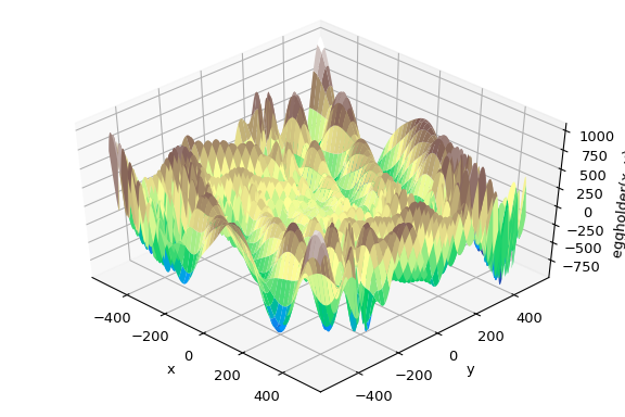
function, namely the (aptly named) eggholder function:
>>> def eggholder(x):
...     return (-(x[1] + 47) * np.sin(np.sqrt(abs(x[0]/2 + (x[1]  + 47))))
...             -x[0] * np.sin(np.sqrt(abs(x[0] - (x[1]  + 47)))))

>>> bounds = [(-512, 512), (-512, 512)]
This function looks like an egg carton:
>>> import matplotlib.pyplot as plt
>>> from mpl_toolkits.mplot3d import Axes3D

>>> x = np.arange(-512, 513)
>>> y = np.arange(-512, 513)
>>> xgrid, ygrid = np.meshgrid(x, y)
>>> xy = np.stack([xgrid, ygrid])

>>> fig = plt.figure()
>>> ax = fig.add_subplot(111, projection='3d')
>>> ax.view_init(45, -45)
>>> ax.plot_surface(xgrid, ygrid, eggholder(xy), cmap='terrain')
>>> ax.set_xlabel('x')
>>> ax.set_ylabel('y')
>>> ax.set_zlabel('eggholder(x, y)')
>>> plt.show()
We now use the global optimizers to obtain the minimum and the function value at the minimum. We’ll store the results in a dictionary so we can compare different optimization results later.
>>> from scipy import optimize
>>> results = dict()
>>> results['shgo'] = optimize.shgo(eggholder, bounds)
>>> results['shgo']
     fun: -935.3379515604197  # may vary
    funl: array([-935.33795156])
 message: 'Optimization terminated successfully.'
    nfev: 42
     nit: 2
   nlfev: 37
   nlhev: 0
   nljev: 9
 success: True
       x: array([439.48096952, 453.97740589])
      xl: array([[439.48096952, 453.97740589]])
>>> results['DA'] = optimize.dual_annealing(eggholder, bounds)
>>> results['DA']
     fun: -956.9182316237413  # may vary
 message: ['Maximum number of iteration reached']
    nfev: 4091
    nhev: 0
     nit: 1000
    njev: 0
       x: array([482.35324114, 432.87892901])
All optimizers return an OptimizeResult, which in addition to the solution
contains information on the number of function evaluations, whether the
optimization was successful, and more. For brevity, we won’t show the full
output of the other optimizers:
>>> results['DE'] = optimize.differential_evolution(eggholder, bounds)
>>> results['BH'] = optimize.basinhopping(eggholder, bounds)
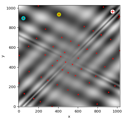
shgo has a second method, which returns all local minima rather than
only what it thinks is the global minimum:
>>> results['shgo_sobol'] = optimize.shgo(eggholder, bounds, n=200, iters=5,
...                                       sampling_method='sobol')
We’ll now plot all found minima on a heatmap of the function:
>>> fig = plt.figure()
>>> ax = fig.add_subplot(111)
>>> im = ax.imshow(eggholder(xy), interpolation='bilinear', origin='lower',
...                cmap='gray')
>>> ax.set_xlabel('x')
>>> ax.set_ylabel('y')
>>>
>>> def plot_point(res, marker='o', color=None):
...     ax.plot(512+res.x[0], 512+res.x[1], marker=marker, color=color, ms=10)

>>> plot_point(results['BH'], color='y')  # basinhopping           - yellow
>>> plot_point(results['DE'], color='c')  # differential_evolution - cyan
>>> plot_point(results['DA'], color='w')  # dual_annealing.        - white

>>> # SHGO produces multiple minima, plot them all (with a smaller marker size)
>>> plot_point(results['shgo'], color='r', marker='+')
>>> plot_point(results['shgo_sobol'], color='r', marker='x')
>>> for i in range(results['shgo_sobol'].xl.shape[0]):
...     ax.plot(512 + results['shgo_sobol'].xl[i, 0],
...             512 + results['shgo_sobol'].xl[i, 1],
...             'ro', ms=2)

>>> ax.set_xlim([-4, 514*2])
>>> ax.set_ylim([-4, 514*2])
>>> plt.show()
Least-squares minimization (least_squares)
SciPy is capable of solving robustified bound-constrained nonlinear least-squares problems:
Here \(f_i(\mathbf{x})\) are smooth functions from \(\mathbb{R}^n\) to \(\mathbb{R}\), we refer to them as residuals. The purpose of a scalar-valued function \(\rho(\cdot)\) is to reduce the influence of outlier residuals and contribute to robustness of the solution, we refer to it as a loss function. A linear loss function gives a standard least-squares problem. Additionally, constraints in a form of lower and upper bounds on some of \(x_j\) are allowed.
All methods specific to least-squares minimization utilize a \(m \times n\)
matrix of partial derivatives called Jacobian and defined as
\(J_{ij} = \partial f_i / \partial x_j\). It is highly recommended to
compute this matrix analytically and pass it to least_squares,
otherwise, it will be estimated by finite differences, which takes a lot of
additional time and can be very inaccurate in hard cases.
Function least_squares can be used for fitting a function
\(\varphi(t; \mathbf{x})\) to empirical data \(\{(t_i, y_i), i = 0, \ldots, m-1\}\).
To do this, one should simply precompute residuals as
\(f_i(\mathbf{x}) = w_i (\varphi(t_i; \mathbf{x}) - y_i)\), where \(w_i\)
are weights assigned to each observation.
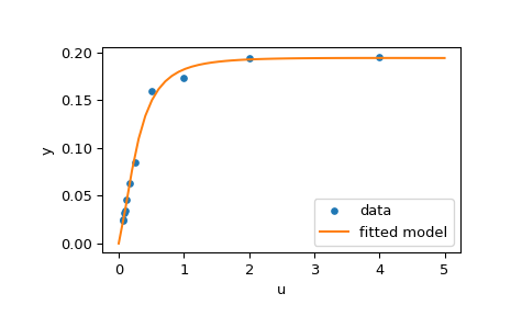
Example of solving a fitting problem
Here we consider an enzymatic reaction 1. There are 11 residuals defined as
where \(y_i\) are measurement values and \(u_i\) are values of the independent variable. The unknown vector of parameters is \(\mathbf{x} = (x_0, x_1, x_2, x_3)^T\). As was said previously, it is recommended to compute Jacobian matrix in a closed form:
We are going to use the “hard” starting point defined in 2. To find a physically meaningful solution, avoid potential division by zero and assure convergence to the global minimum we impose constraints \(0 \leq x_j \leq 100, j = 0, 1, 2, 3\).
The code below implements least-squares estimation of \(\mathbf{x}\) and finally plots the original data and the fitted model function:
>>> from scipy.optimize import least_squares
>>> def model(x, u):
...     return x[0] * (u ** 2 + x[1] * u) / (u ** 2 + x[2] * u + x[3])
>>> def fun(x, u, y):
...     return model(x, u) - y
>>> def jac(x, u, y):
...     J = np.empty((u.size, x.size))
...     den = u ** 2 + x[2] * u + x[3]
...     num = u ** 2 + x[1] * u
...     J[:, 0] = num / den
...     J[:, 1] = x[0] * u / den
...     J[:, 2] = -x[0] * num * u / den ** 2
...     J[:, 3] = -x[0] * num / den ** 2
...     return J
>>> u = np.array([4.0, 2.0, 1.0, 5.0e-1, 2.5e-1, 1.67e-1, 1.25e-1, 1.0e-1,
...               8.33e-2, 7.14e-2, 6.25e-2])
>>> y = np.array([1.957e-1, 1.947e-1, 1.735e-1, 1.6e-1, 8.44e-2, 6.27e-2,
...               4.56e-2, 3.42e-2, 3.23e-2, 2.35e-2, 2.46e-2])
>>> x0 = np.array([2.5, 3.9, 4.15, 3.9])
>>> res = least_squares(fun, x0, jac=jac, bounds=(0, 100), args=(u, y), verbose=1)
# may vary
`ftol` termination condition is satisfied.
Function evaluations 130, initial cost 4.4383e+00, final cost 1.5375e-04, first-order optimality 4.92e-08.
>>> res.x
array([ 0.19280596,  0.19130423,  0.12306063,  0.13607247])
>>> import matplotlib.pyplot as plt
>>> u_test = np.linspace(0, 5)
>>> y_test = model(res.x, u_test)
>>> plt.plot(u, y, 'o', markersize=4, label='data')
>>> plt.plot(u_test, y_test, label='fitted model')
>>> plt.xlabel("u")
>>> plt.ylabel("y")
>>> plt.legend(loc='lower right')
>>> plt.show()
Further examples
Three interactive examples below illustrate usage of least_squares in
greater detail.
Large-scale bundle adjustment in scipy demonstrates large-scale capabilities of
least_squaresand how to efficiently compute finite difference approximation of sparse Jacobian.Robust nonlinear regression in scipy shows how to handle outliers with a robust loss function in a nonlinear regression.
Solving a discrete boundary-value problem in scipy examines how to solve a large system of equations and use bounds to achieve desired properties of the solution.
For the details about mathematical algorithms behind the implementation refer
to documentation of least_squares.
Univariate function minimizers (minimize_scalar)
Often only the minimum of an univariate function (i.e., a function that
takes a scalar as input) is needed. In these circumstances, other
optimization techniques have been developed that can work faster. These are
accessible from the minimize_scalar function, which proposes several
algorithms.
Unconstrained minimization (method='brent')
There are, actually, two methods that can be used to minimize an univariate
function: brent and golden, but golden is included only for academic
purposes and should rarely be used. These can be respectively selected
through the method parameter in minimize_scalar. The brent
method uses Brent’s algorithm for locating a minimum. Optimally, a bracket
(the bracket parameter) should be given which contains the minimum desired. A
bracket is a triple \(\left( a, b, c \right)\) such that \(f
\left( a \right) > f \left( b \right) < f \left( c \right)\) and \(a <
b < c\) . If this is not given, then alternatively two starting points can
be chosen and a bracket will be found from these points using a simple
marching algorithm. If these two starting points are not provided, 0 and
1 will be used (this may not be the right choice for your function and
result in an unexpected minimum being returned).
Here is an example:
>>> from scipy.optimize import minimize_scalar
>>> f = lambda x: (x - 2) * (x + 1)**2
>>> res = minimize_scalar(f, method='brent')
>>> print(res.x)
1.0
Bounded minimization (method='bounded')
Very often, there are constraints that can be placed on the solution space
before minimization occurs. The bounded method in minimize_scalar
is an example of a constrained minimization procedure that provides a
rudimentary interval constraint for scalar functions. The interval
constraint allows the minimization to occur only between two fixed
endpoints, specified using the mandatory bounds parameter.
For example, to find the minimum of \(J_{1}\left( x \right)\) near
\(x=5\) , minimize_scalar can be called using the interval
\(\left[ 4, 7 \right]\) as a constraint. The result is
\(x_{\textrm{min}}=5.3314\) :
>>> from scipy.special import j1
>>> res = minimize_scalar(j1, bounds=(4, 7), method='bounded')
>>> res.x
5.33144184241
Custom minimizers
Sometimes, it may be useful to use a custom method as a (multivariate
or univariate) minimizer, for example, when using some library wrappers
of minimize (e.g., basinhopping).
We can achieve that by, instead of passing a method name, passing a callable (either a function or an object implementing a __call__ method) as the method parameter.
Let us consider an (admittedly rather virtual) need to use a trivial custom multivariate minimization method that will just search the neighborhood in each dimension independently with a fixed step size:
>>> from scipy.optimize import OptimizeResult
>>> def custmin(fun, x0, args=(), maxfev=None, stepsize=0.1,
...         maxiter=100, callback=None, **options):
...     bestx = x0
...     besty = fun(x0)
...     funcalls = 1
...     niter = 0
...     improved = True
...     stop = False
...
...     while improved and not stop and niter < maxiter:
...         improved = False
...         niter += 1
...         for dim in range(np.size(x0)):
...             for s in [bestx[dim] - stepsize, bestx[dim] + stepsize]:
...                 testx = np.copy(bestx)
...                 testx[dim] = s
...                 testy = fun(testx, *args)
...                 funcalls += 1
...                 if testy < besty:
...                     besty = testy
...                     bestx = testx
...                     improved = True
...             if callback is not None:
...                 callback(bestx)
...             if maxfev is not None and funcalls >= maxfev:
...                 stop = True
...                 break
...
...     return OptimizeResult(fun=besty, x=bestx, nit=niter,
...                           nfev=funcalls, success=(niter > 1))
>>> x0 = [1.35, 0.9, 0.8, 1.1, 1.2]
>>> res = minimize(rosen, x0, method=custmin, options=dict(stepsize=0.05))
>>> res.x
array([1., 1., 1., 1., 1.])
This will work just as well in case of univariate optimization:
>>> def custmin(fun, bracket, args=(), maxfev=None, stepsize=0.1,
...         maxiter=100, callback=None, **options):
...     bestx = (bracket[1] + bracket[0]) / 2.0
...     besty = fun(bestx)
...     funcalls = 1
...     niter = 0
...     improved = True
...     stop = False
...
...     while improved and not stop and niter < maxiter:
...         improved = False
...         niter += 1
...         for testx in [bestx - stepsize, bestx + stepsize]:
...             testy = fun(testx, *args)
...             funcalls += 1
...             if testy < besty:
...                 besty = testy
...                 bestx = testx
...                 improved = True
...         if callback is not None:
...             callback(bestx)
...         if maxfev is not None and funcalls >= maxfev:
...             stop = True
...             break
...
...     return OptimizeResult(fun=besty, x=bestx, nit=niter,
...                           nfev=funcalls, success=(niter > 1))
>>> def f(x):
...    return (x - 2)**2 * (x + 2)**2
>>> res = minimize_scalar(f, bracket=(-3.5, 0), method=custmin,
...                       options=dict(stepsize = 0.05))
>>> res.x
-2.0
Root finding
Scalar functions
If one has a single-variable equation, there are multiple different root
finding algorithms that can be tried. Most of these algorithms require the
endpoints of an interval in which a root is expected (because the function
changes signs). In general, brentq is the best choice, but the other
methods may be useful in certain circumstances or for academic purposes.
When a bracket is not available, but one or more derivatives are available,
then newton (or halley, secant) may be applicable.
This is especially the case if the function is defined on a subset of the
complex plane, and the bracketing methods cannot be used.
Fixed-point solving
A problem closely related to finding the zeros of a function is the
problem of finding a fixed point of a function. A fixed point of a
function is the point at which evaluation of the function returns the
point: \(g\left(x\right)=x.\) Clearly, the fixed point of \(g\)
is the root of \(f\left(x\right)=g\left(x\right)-x.\)
Equivalently, the root of \(f\) is the fixed point of
\(g\left(x\right)=f\left(x\right)+x.\) The routine
fixed_point provides a simple iterative method using Aitkens
sequence acceleration to estimate the fixed point of \(g\) given a
starting point.
Sets of equations
Finding a root of a set of non-linear equations can be achieved using the
root function. Several methods are available, amongst which hybr
(the default) and lm, which, respectively, use the hybrid method of Powell
and the Levenberg-Marquardt method from MINPACK.
The following example considers the single-variable transcendental equation
a root of which can be found as follows:
>>> import numpy as np
>>> from scipy.optimize import root
>>> def func(x):
...     return x + 2 * np.cos(x)
>>> sol = root(func, 0.3)
>>> sol.x
array([-1.02986653])
>>> sol.fun
array([ -6.66133815e-16])
Consider now a set of non-linear equations
We define the objective function so that it also returns the Jacobian and
indicate this by setting the jac parameter to True. Also, the
Levenberg-Marquardt solver is used here.
>>> def func2(x):
...     f = [x[0] * np.cos(x[1]) - 4,
...          x[1]*x[0] - x[1] - 5]
...     df = np.array([[np.cos(x[1]), -x[0] * np.sin(x[1])],
...                    [x[1], x[0] - 1]])
...     return f, df
>>> sol = root(func2, [1, 1], jac=True, method='lm')
>>> sol.x
array([ 6.50409711,  0.90841421])
Root finding for large problems
Methods hybr and lm in root cannot deal with a very large
number of variables (N), as they need to calculate and invert a dense N
x N Jacobian matrix on every Newton step. This becomes rather inefficient
when N grows.
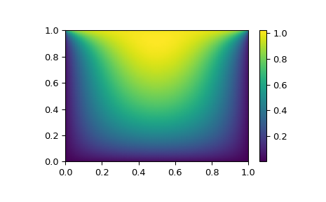
Consider, for instance, the following problem: we need to solve the following integrodifferential equation on the square \([0,1]\times[0,1]\):
with the boundary condition \(P(x,1) = 1\) on the upper edge and
\(P=0\) elsewhere on the boundary of the square. This can be done
by approximating the continuous function P by its values on a grid,
\(P_{n,m}\approx{}P(n h, m h)\), with a small grid spacing
h. The derivatives and integrals can then be approximated; for
instance \(\partial_x^2 P(x,y)\approx{}(P(x+h,y) - 2 P(x,y) +
P(x-h,y))/h^2\). The problem is then equivalent to finding the root of
some function residual(P), where P is a vector of length
\(N_x N_y\).
Now, because \(N_x N_y\) can be large, methods hybr or lm in
root will take a long time to solve this problem. The solution can,
however, be found using one of the large-scale solvers, for example
krylov, broyden2, or anderson. These use what is known as the
inexact Newton method, which instead of computing the Jacobian matrix
exactly, forms an approximation for it.
The problem we have can now be solved as follows:
import numpy as np
from scipy.optimize import root
from numpy import cosh, zeros_like, mgrid, zeros

# parameters
nx, ny = 75, 75
hx, hy = 1./(nx-1), 1./(ny-1)

P_left, P_right = 0, 0
P_top, P_bottom = 1, 0

def residual(P):
   d2x = zeros_like(P)
   d2y = zeros_like(P)

   d2x[1:-1] = (P[2:]   - 2*P[1:-1] + P[:-2]) / hx/hx
   d2x[0]    = (P[1]    - 2*P[0]    + P_left)/hx/hx
   d2x[-1]   = (P_right - 2*P[-1]   + P[-2])/hx/hx

   d2y[:,1:-1] = (P[:,2:] - 2*P[:,1:-1] + P[:,:-2])/hy/hy
   d2y[:,0]    = (P[:,1]  - 2*P[:,0]    + P_bottom)/hy/hy
   d2y[:,-1]   = (P_top   - 2*P[:,-1]   + P[:,-2])/hy/hy

   return d2x + d2y + 5*cosh(P).mean()**2

# solve
guess = zeros((nx, ny), float)
sol = root(residual, guess, method='krylov', options={'disp': True})
#sol = root(residual, guess, method='broyden2', options={'disp': True, 'max_rank': 50})
#sol = root(residual, guess, method='anderson', options={'disp': True, 'M': 10})
print('Residual: %g' % abs(residual(sol.x)).max())

# visualize
import matplotlib.pyplot as plt
x, y = mgrid[0:1:(nx*1j), 0:1:(ny*1j)]
plt.pcolormesh(x, y, sol.x, shading='gouraud')
plt.colorbar()
plt.show()
Still too slow? Preconditioning.
When looking for the zero of the functions \(f_i({\bf x}) = 0\),
i = 1, 2, …, N, the krylov solver spends most of the
time inverting the Jacobian matrix,
If you have an approximation for the inverse matrix \(M\approx{}J^{-1}\), you can use it for preconditioning the linear-inversion problem. The idea is that instead of solving \(J{\bf s}={\bf y}\) one solves \(MJ{\bf s}=M{\bf y}\): since matrix \(MJ\) is “closer” to the identity matrix than \(J\) is, the equation should be easier for the Krylov method to deal with.
The matrix M can be passed to root with method krylov as an
option options['jac_options']['inner_M']. It can be a (sparse) matrix
or a scipy.sparse.linalg.LinearOperator instance.
For the problem in the previous section, we note that the function to solve consists of two parts: the first one is the application of the Laplace operator, \([\partial_x^2 + \partial_y^2] P\), and the second is the integral. We can actually easily compute the Jacobian corresponding to the Laplace operator part: we know that in 1-D
so that the whole 2-D operator is represented by
The matrix \(J_2\) of the Jacobian corresponding to the integral
is more difficult to calculate, and since all of it entries are
nonzero, it will be difficult to invert. \(J_1\) on the other hand
is a relatively simple matrix, and can be inverted by
scipy.sparse.linalg.splu (or the inverse can be approximated by
scipy.sparse.linalg.spilu). So we are content to take
\(M\approx{}J_1^{-1}\) and hope for the best.
In the example below, we use the preconditioner \(M=J_1^{-1}\).
import numpy as np
from scipy.optimize import root
from scipy.sparse import spdiags, kron
from scipy.sparse.linalg import spilu, LinearOperator
from numpy import cosh, zeros_like, mgrid, zeros, eye

# parameters
nx, ny = 75, 75
hx, hy = 1./(nx-1), 1./(ny-1)

P_left, P_right = 0, 0
P_top, P_bottom = 1, 0

def get_preconditioner():
    """Compute the preconditioner M"""
    diags_x = zeros((3, nx))
    diags_x[0,:] = 1/hx/hx
    diags_x[1,:] = -2/hx/hx
    diags_x[2,:] = 1/hx/hx
    Lx = spdiags(diags_x, [-1,0,1], nx, nx)

    diags_y = zeros((3, ny))
    diags_y[0,:] = 1/hy/hy
    diags_y[1,:] = -2/hy/hy
    diags_y[2,:] = 1/hy/hy
    Ly = spdiags(diags_y, [-1,0,1], ny, ny)

    J1 = kron(Lx, eye(ny)) + kron(eye(nx), Ly)

    # Now we have the matrix `J_1`. We need to find its inverse `M` --
    # however, since an approximate inverse is enough, we can use
    # the *incomplete LU* decomposition

    J1_ilu = spilu(J1)

    # This returns an object with a method .solve() that evaluates
    # the corresponding matrix-vector product. We need to wrap it into
    # a LinearOperator before it can be passed to the Krylov methods:

    M = LinearOperator(shape=(nx*ny, nx*ny), matvec=J1_ilu.solve)
    return M

def solve(preconditioning=True):
    """Compute the solution"""
    count = [0]

    def residual(P):
        count[0] += 1

        d2x = zeros_like(P)
        d2y = zeros_like(P)

        d2x[1:-1] = (P[2:]   - 2*P[1:-1] + P[:-2])/hx/hx
        d2x[0]    = (P[1]    - 2*P[0]    + P_left)/hx/hx
        d2x[-1]   = (P_right - 2*P[-1]   + P[-2])/hx/hx

        d2y[:,1:-1] = (P[:,2:] - 2*P[:,1:-1] + P[:,:-2])/hy/hy
        d2y[:,0]    = (P[:,1]  - 2*P[:,0]    + P_bottom)/hy/hy
        d2y[:,-1]   = (P_top   - 2*P[:,-1]   + P[:,-2])/hy/hy

        return d2x + d2y + 5*cosh(P).mean()**2

    # preconditioner
    if preconditioning:
        M = get_preconditioner()
    else:
        M = None

    # solve
    guess = zeros((nx, ny), float)

    sol = root(residual, guess, method='krylov',
               options={'disp': True,
                        'jac_options': {'inner_M': M}})
    print('Residual', abs(residual(sol.x)).max())
    print('Evaluations', count[0])

    return sol.x

def main():
    sol = solve(preconditioning=True)

    # visualize
    import matplotlib.pyplot as plt
    x, y = mgrid[0:1:(nx*1j), 0:1:(ny*1j)]
    plt.clf()
    plt.pcolor(x, y, sol)
    plt.clim(0, 1)
    plt.colorbar()
    plt.show()


if __name__ == "__main__":
    main()
Resulting run, first without preconditioning:
0:  |F(x)| = 803.614; step 1; tol 0.000257947
1:  |F(x)| = 345.912; step 1; tol 0.166755
2:  |F(x)| = 139.159; step 1; tol 0.145657
3:  |F(x)| = 27.3682; step 1; tol 0.0348109
4:  |F(x)| = 1.03303; step 1; tol 0.00128227
5:  |F(x)| = 0.0406634; step 1; tol 0.00139451
6:  |F(x)| = 0.00344341; step 1; tol 0.00645373
7:  |F(x)| = 0.000153671; step 1; tol 0.00179246
8:  |F(x)| = 6.7424e-06; step 1; tol 0.00173256
Residual 3.57078908664e-07
Evaluations 317
and then with preconditioning:
0:  |F(x)| = 136.993; step 1; tol 7.49599e-06
1:  |F(x)| = 4.80983; step 1; tol 0.00110945
2:  |F(x)| = 0.195942; step 1; tol 0.00149362
3:  |F(x)| = 0.000563597; step 1; tol 7.44604e-06
4:  |F(x)| = 1.00698e-09; step 1; tol 2.87308e-12
Residual 9.29603061195e-11
Evaluations 77
Using a preconditioner reduced the number of evaluations of the
residual function by a factor of 4. For problems where the
residual is expensive to compute, good preconditioning can be crucial
— it can even decide whether the problem is solvable in practice or
not.
Preconditioning is an art, science, and industry. Here, we were lucky in making a simple choice that worked reasonably well, but there is a lot more depth to this topic than is shown here.
Linear programming (linprog)
The function linprog can minimize a linear objective function
subject to linear equality and inequality constraints. This kind of
problem is well known as linear programming. Linear programming solves
problems of the following form:
where \(x\) is a vector of decision variables; \(c\), \(b_{ub}\), \(b_{eq}\), \(l\), and \(u\) are vectors; and \(A_{ub}\) and \(A_{eq}\) are matrices.
In this tutorial, we will try to solve a typical linear programming
problem using linprog.
Linear programming example
Consider the following simple linear programming problem:
We need some mathematical manipulations to convert the target problem to the form accepted by linprog.
First of all, let’s consider the objective function.
We want to maximize the objective
function, but linprog can only accept a minimization problem. This is easily remedied by converting the maximize
\(29x_1 + 45x_2\) to minimizing \(-29x_1 -45x_2\). Also, \(x_3, x_4\) are not shown in the objective
function. That means the weights corresponding with \(x_3, x_4\) are zero. So, the objective function can be
converted to:
If we define the vector of decision variables \(x = [x_1, x_2, x_3, x_4]^T\), the objective weights vector \(c\) of linprog in this problem
should be
Next, let’s consider the two inequality constraints. The first one is a “less than” inequality, so it is already in the form accepted by linprog.
The second one is a “greater than” inequality, so we need to multiply both sides by \(-1\) to convert it to a “less than” inequality.
Explicitly showing zero coefficients, we have:
These equations can be converted to matrix form:
where
Next, let’s consider the two equality constraints. Showing zero weights explicitly, these are:
These equations can be converted to matrix form:
where
Lastly, let’s consider the separate inequality constraints on individual decision variables, which are known as
“box constraints” or “simple bounds”. These constraints can be applied using the bounds argument of linprog.
As noted in the linprog documentation, the default value of bounds is (0, None), meaning that the
lower bound on each decision variable is 0, and the upper bound on each decision variable is infinity:
all the decision variables are non-negative. Our bounds are different, so we will need to specify the lower and upper bound on each
decision variable as a tuple and group these tuples into a list.
Finally, we can solve the transformed problem using linprog.
>>> import numpy as np
>>> from scipy.optimize import linprog
>>> c = np.array([-29.0, -45.0, 0.0, 0.0])
>>> A_ub = np.array([[1.0, -1.0, -3.0, 0.0],
...                 [-2.0, 3.0, 7.0, -3.0]])
>>> b_ub = np.array([5.0, -10.0])
>>> A_eq = np.array([[2.0, 8.0, 1.0, 0.0],
...                 [4.0, 4.0, 0.0, 1.0]])
>>> b_eq = np.array([60.0, 60.0])
>>> x0_bounds = (0, None)
>>> x1_bounds = (0, 5.0)
>>> x2_bounds = (-np.inf, 0.5)  # +/- np.inf can be used instead of None
>>> x3_bounds = (-3.0, None)
>>> bounds = [x0_bounds, x1_bounds, x2_bounds, x3_bounds]
>>> result = linprog(c, A_ub=A_ub, b_ub=b_ub, A_eq=A_eq, b_eq=b_eq, bounds=bounds)
>>> print(result)
     con: array([15.5361242 , 16.61288005])  # may vary
     fun: -370.2321976308326  # may vary
 message: 'The algorithm terminated successfully and determined that the problem is infeasible.'
     nit: 6  # may vary
   slack: array([ 0.79314989, -1.76308532])  # may vary
  status: 2
 success: False
       x: array([ 6.60059391,  3.97366609, -0.52664076,  1.09007993])  # may vary
The result states that our problem is infeasible, meaning that there is no solution vector that satisfies all the
constraints. That doesn’t necessarily mean we did anything wrong; some problems truly are infeasible.
Suppose, however, that we were to decide that our bound constraint on \(x_1\) was too tight and that it could be loosened
to \(0 \leq x_1 \leq 6\). After adjusting our code x1_bounds = (0, 6) to reflect the change and executing it again:
>>> x1_bounds = (0, 6)
>>> bounds = [x0_bounds, x1_bounds, x2_bounds, x3_bounds]
>>> result = linprog(c, A_ub=A_ub, b_ub=b_ub, A_eq=A_eq, b_eq=b_eq, bounds=bounds)
>>> print(result)
    con: array([9.78840831e-09, 1.04662945e-08])  # may vary
    fun: -505.97435889013434  # may vary
message: 'Optimization terminated successfully.'
    nit: 4  # may vary
  slack: array([ 6.52747190e-10, -2.26730279e-09])  # may vary
 status: 0
success: True
      x: array([ 9.41025641,  5.17948718, -0.25641026,  1.64102564])  # may vary
The result shows the optimization was successful.
We can check the objective value (result.fun) is same as \(c^Tx\):
>>> x = np.array(result.x)
>>> print(c @ x)
-505.97435889013434  # may vary
We can also check that all constraints are satisfied within reasonable tolerances:
>>> print(b_ub - (A_ub @ x).flatten())  # this is equivalent to result.slack
[ 6.52747190e-10, -2.26730279e-09]  # may vary
>>> print(b_eq - (A_eq @ x).flatten())  # this is equivalent to result.con
[ 9.78840831e-09, 1.04662945e-08]]  # may vary
>>> print([0 <= result.x[0], 0 <= result.x[1] <= 6.0, result.x[2] <= 0.5, -3.0 <= result.x[3]])
[True, True, True, True]
If we need greater accuracy, typically at the expense of speed, we can solve using the revised simplex method:
>>> result = linprog(c, A_ub=A_ub, b_ub=b_ub, A_eq=A_eq, b_eq=b_eq, bounds=bounds, method='revised simplex')
>>> print(result)
    con: array([0.00000000e+00, 7.10542736e-15])  # may vary
    fun: -505.97435897435895    # may vary
message: 'Optimization terminated successfully.'
    nit: 5  # may vary
  slack: array([ 1.77635684e-15, -3.55271368e-15])  # may vary
 status: 0
success: True
      x: array([ 9.41025641,  5.17948718, -0.25641026,  1.64102564])  # may vary
References
Some further reading and related software, such as Newton-Krylov [KK], PETSc [PP], and PyAMG [AMG]:
- KK
D.A. Knoll and D.E. Keyes, “Jacobian-free Newton-Krylov methods”, J. Comp. Phys. 193, 357 (2004). doi:10.1016/j.jcp.2003.08.010
- PP
PETSc https://www.mcs.anl.gov/petsc/ and its Python bindings https://bitbucket.org/petsc/petsc4py/
- AMG
PyAMG (algebraic multigrid preconditioners/solvers) https://github.com/pyamg/pyamg/issues