scipy.stats.moyal
-
scipy.stats.moyal(*args, **kwds) = <scipy.stats._continuous_distns.moyal_gen object>[source]¶ A Moyal continuous random variable.
As an instance of the
rv_continuousclass,moyalobject inherits from it a collection of generic methods (see below for the full list), and completes them with details specific for this particular distribution.Notes
The probability density function for
moyalis:\[f(x) = \exp(-(x + \exp(-x))/2) / \sqrt{2\pi}\]for a real number \(x\).
The probability density above is defined in the “standardized” form. To shift and/or scale the distribution use the
locandscaleparameters. Specifically,moyal.pdf(x, loc, scale)is identically equivalent tomoyal.pdf(y) / scalewithy = (x - loc) / scale.This distribution has utility in high-energy physics and radiation detection. It describes the energy loss of a charged relativistic particle due to ionization of the medium [1]. It also provides an approximation for the Landau distribution. For an in depth description see [2]. For additional description, see [3].
References
- 1
J.E. Moyal, “XXX. Theory of ionization fluctuations”, The London, Edinburgh, and Dublin Philosophical Magazine and Journal of Science, vol 46, 263-280, (1955). DOI:10.1080/14786440308521076 (gated)
- 2
G. Cordeiro et al., “The beta Moyal: a useful skew distribution”, International Journal of Research and Reviews in Applied Sciences, vol 10, 171-192, (2012). http://www.arpapress.com/Volumes/Vol10Issue2/IJRRAS_10_2_02.pdf
- 3
C. Walck, “Handbook on Statistical Distributions for Experimentalists; International Report SUF-PFY/96-01”, Chapter 26, University of Stockholm: Stockholm, Sweden, (2007). http://www.stat.rice.edu/~dobelman/textfiles/DistributionsHandbook.pdf
New in version 1.1.0.
Examples
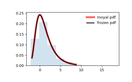
>>> from scipy.stats import moyal
>>> import matplotlib.pyplot as plt
>>> fig, ax = plt.subplots(1, 1)
Calculate a few first moments:
>>> mean, var, skew, kurt = moyal.stats(moments='mvsk')
Display the probability density function (
pdf):>>> x = np.linspace(moyal.ppf(0.01), ... moyal.ppf(0.99), 100) >>> ax.plot(x, moyal.pdf(x), ... 'r-', lw=5, alpha=0.6, label='moyal pdf')
Alternatively, the distribution object can be called (as a function) to fix the shape, location and scale parameters. This returns a “frozen” RV object holding the given parameters fixed.
Freeze the distribution and display the frozen
pdf:>>> rv = moyal() >>> ax.plot(x, rv.pdf(x), 'k-', lw=2, label='frozen pdf')
Check accuracy of
cdfandppf:>>> vals = moyal.ppf([0.001, 0.5, 0.999]) >>> np.allclose([0.001, 0.5, 0.999], moyal.cdf(vals)) True
Generate random numbers:
>>> r = moyal.rvs(size=1000)
And compare the histogram:
>>> ax.hist(r, density=True, histtype='stepfilled', alpha=0.2)
>>> ax.legend(loc='best', frameon=False)
>>> plt.show()
Methods
rvs(loc=0, scale=1, size=1, random_state=None)
Random variates.
pdf(x, loc=0, scale=1)
Probability density function.
logpdf(x, loc=0, scale=1)
Log of the probability density function.
cdf(x, loc=0, scale=1)
Cumulative distribution function.
logcdf(x, loc=0, scale=1)
Log of the cumulative distribution function.
sf(x, loc=0, scale=1)
Survival function (also defined as
1 - cdf, but sf is sometimes more accurate).logsf(x, loc=0, scale=1)
Log of the survival function.
ppf(q, loc=0, scale=1)
Percent point function (inverse of
cdf— percentiles).isf(q, loc=0, scale=1)
Inverse survival function (inverse of
sf).moment(n, loc=0, scale=1)
Non-central moment of order n
stats(loc=0, scale=1, moments=’mv’)
Mean(‘m’), variance(‘v’), skew(‘s’), and/or kurtosis(‘k’).
entropy(loc=0, scale=1)
(Differential) entropy of the RV.
fit(data)
Parameter estimates for generic data. See scipy.stats.rv_continuous.fit for detailed documentation of the keyword arguments.
expect(func, args=(), loc=0, scale=1, lb=None, ub=None, conditional=False, **kwds)
Expected value of a function (of one argument) with respect to the distribution.
median(loc=0, scale=1)
Median of the distribution.
mean(loc=0, scale=1)
Mean of the distribution.
var(loc=0, scale=1)
Variance of the distribution.
std(loc=0, scale=1)
Standard deviation of the distribution.
interval(alpha, loc=0, scale=1)
Endpoints of the range that contains alpha percent of the distribution