scipy.signal.windows.general_hamming

scipy.signal.windows.general_hamming(M, alpha, sym=True)

Return a generalized Hamming window.

The generalized Hamming window is constructed by multiplying a rectangular window by one period of a cosine function [1].

Parameters

Mint

Number of points in the output window. If zero or less, an empty array is returned.

alphafloat

The window coefficient, \(\alpha\)

symbool, optional

When True (default), generates a symmetric window, for use in filter design. When False, generates a periodic window, for use in spectral analysis.

Returns

wndarray

The window, with the maximum value normalized to 1 (though the value 1 does not appear if M is even and sym is True).

See also

hamming, hann

Notes

The generalized Hamming window is defined as

\[w(n) = \alpha - \left(1 - \alpha\right) \cos\left(\frac{2\pi{n}}{M-1}\right) \qquad 0 \leq n \leq M-1\]

Both the common Hamming window and Hann window are special cases of the generalized Hamming window with \(\alpha\) = 0.54 and \(\alpha\) = 0.5, respectively [2].

References

1

DSPRelated, “Generalized Hamming Window Family”, https://www.dsprelated.com/freebooks/sasp/Generalized_Hamming_Window_Family.html

2

Wikipedia, “Window function”, https://en.wikipedia.org/wiki/Window_function

3

Riccardo Piantanida ESA, “Sentinel-1 Level 1 Detailed Algorithm Definition”, https://sentinel.esa.int/documents/247904/1877131/Sentinel-1-Level-1-Detailed-Algorithm-Definition

4

Matthieu Bourbigot ESA, “Sentinel-1 Product Definition”, https://sentinel.esa.int/documents/247904/1877131/Sentinel-1-Product-Definition

Examples

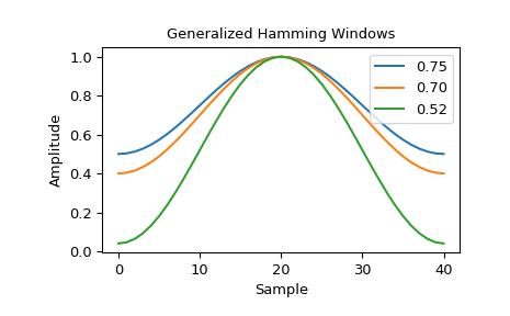
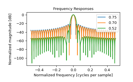
The Sentinel-1A/B Instrument Processing Facility uses generalized Hamming windows in the processing of spaceborne Synthetic Aperture Radar (SAR) data [3]. The facility uses various values for the \(\alpha\) parameter based on operating mode of the SAR instrument. Some common \(\alpha\) values include 0.75, 0.7 and 0.52 [4]. As an example, we plot these different windows.

>>> from scipy.signal.windows import general_hamming
>>> from scipy.fft import fft, fftshift
>>> import matplotlib.pyplot as plt

>>> fig1, spatial_plot = plt.subplots()
>>> spatial_plot.set_title("Generalized Hamming Windows")
>>> spatial_plot.set_ylabel("Amplitude")
>>> spatial_plot.set_xlabel("Sample")

>>> fig2, freq_plot = plt.subplots()
>>> freq_plot.set_title("Frequency Responses")
>>> freq_plot.set_ylabel("Normalized magnitude [dB]")
>>> freq_plot.set_xlabel("Normalized frequency [cycles per sample]")

>>> for alpha in [0.75, 0.7, 0.52]:
...     window = general_hamming(41, alpha)
...     spatial_plot.plot(window, label="{:.2f}".format(alpha))
...     A = fft(window, 2048) / (len(window)/2.0)
...     freq = np.linspace(-0.5, 0.5, len(A))
...     response = 20 * np.log10(np.abs(fftshift(A / abs(A).max())))
...     freq_plot.plot(freq, response, label="{:.2f}".format(alpha))
>>> freq_plot.legend(loc="upper right")
>>> spatial_plot.legend(loc="upper right")