scipy.signal.iirfilter
-
scipy.signal.iirfilter(N, Wn, rp=None, rs=None, btype='band', analog=False, ftype='butter', output='ba', fs=None)[source]¶ IIR digital and analog filter design given order and critical points.
Design an Nth-order digital or analog filter and return the filter coefficients.
- Parameters
- Nint
The order of the filter.
- Wnarray_like
A scalar or length-2 sequence giving the critical frequencies.
For digital filters, Wn are in the same units as fs. By default, fs is 2 half-cycles/sample, so these are normalized from 0 to 1, where 1 is the Nyquist frequency. (Wn is thus in half-cycles / sample.)
For analog filters, Wn is an angular frequency (e.g. rad/s).
- rpfloat, optional
For Chebyshev and elliptic filters, provides the maximum ripple in the passband. (dB)
- rsfloat, optional
For Chebyshev and elliptic filters, provides the minimum attenuation in the stop band. (dB)
- btype{‘bandpass’, ‘lowpass’, ‘highpass’, ‘bandstop’}, optional
The type of filter. Default is ‘bandpass’.
- analogbool, optional
When True, return an analog filter, otherwise a digital filter is returned.
- ftypestr, optional
The type of IIR filter to design:
Butterworth : ‘butter’
Chebyshev I : ‘cheby1’
Chebyshev II : ‘cheby2’
Cauer/elliptic: ‘ellip’
Bessel/Thomson: ‘bessel’
- output{‘ba’, ‘zpk’, ‘sos’}, optional
Type of output: numerator/denominator (‘ba’), pole-zero (‘zpk’), or second-order sections (‘sos’). Default is ‘ba’.
- fsfloat, optional
The sampling frequency of the digital system.
New in version 1.2.0.
- Returns
- b, andarray, ndarray
Numerator (b) and denominator (a) polynomials of the IIR filter. Only returned if
output='ba'.- z, p, kndarray, ndarray, float
Zeros, poles, and system gain of the IIR filter transfer function. Only returned if
output='zpk'.- sosndarray
Second-order sections representation of the IIR filter. Only returned if
output=='sos'.
See also
Notes
The
'sos'output parameter was added in 0.16.0.Examples
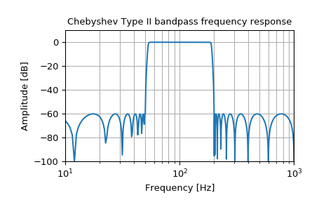
Generate a 17th-order Chebyshev II analog bandpass filter from 50 Hz to 200 Hz and plot the frequency response:
>>> from scipy import signal
>>> import matplotlib.pyplot as plt
>>> b, a = signal.iirfilter(17, [2*np.pi*50, 2*np.pi*200], rs=60,
...                         btype='band', analog=True, ftype='cheby2')
>>> w, h = signal.freqs(b, a, 1000)
>>> fig = plt.figure()
>>> ax = fig.add_subplot(1, 1, 1)
>>> ax.semilogx(w / (2*np.pi), 20 * np.log10(np.maximum(abs(h), 1e-5)))
>>> ax.set_title('Chebyshev Type II bandpass frequency response')
>>> ax.set_xlabel('Frequency [Hz]')
>>> ax.set_ylabel('Amplitude [dB]')
>>> ax.axis((10, 1000, -100, 10))
>>> ax.grid(which='both', axis='both')
>>> plt.show()
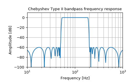
Create a digital filter with the same properties, in a system with sampling rate of 2000 Hz, and plot the frequency response. (Second-order sections implementation is required to ensure stability of a filter of this order):
>>> sos = signal.iirfilter(17, [50, 200], rs=60, btype='band',
...                        analog=False, ftype='cheby2', fs=2000,
...                        output='sos')
>>> w, h = signal.sosfreqz(sos, 2000, fs=2000)
>>> fig = plt.figure()
>>> ax = fig.add_subplot(1, 1, 1)
>>> ax.semilogx(w, 20 * np.log10(np.maximum(abs(h), 1e-5)))
>>> ax.set_title('Chebyshev Type II bandpass frequency response')
>>> ax.set_xlabel('Frequency [Hz]')
>>> ax.set_ylabel('Amplitude [dB]')
>>> ax.axis((10, 1000, -100, 10))
>>> ax.grid(which='both', axis='both')
>>> plt.show()