scipy.signal.fftconvolve
-
scipy.signal.fftconvolve(in1, in2, mode='full', axes=None)[source]¶ Convolve two N-dimensional arrays using FFT.
Convolve in1 and in2 using the fast Fourier transform method, with the output size determined by the mode argument.
This is generally much faster than
convolvefor large arrays (n > ~500), but can be slower when only a few output values are needed, and can only output float arrays (int or object array inputs will be cast to float).As of v0.19,
convolveautomatically chooses this method or the direct method based on an estimation of which is faster.- Parameters
- in1array_like
First input.
- in2array_like
Second input. Should have the same number of dimensions as in1.
- modestr {‘full’, ‘valid’, ‘same’}, optional
A string indicating the size of the output:
fullThe output is the full discrete linear convolution of the inputs. (Default)
validThe output consists only of those elements that do not rely on the zero-padding. In ‘valid’ mode, either in1 or in2 must be at least as large as the other in every dimension.
sameThe output is the same size as in1, centered with respect to the ‘full’ output. axis : tuple, optional
- axesint or array_like of ints or None, optional
Axes over which to compute the convolution. The default is over all axes.
- Returns
- outarray
An N-dimensional array containing a subset of the discrete linear convolution of in1 with in2.
Examples
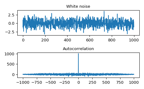
Autocorrelation of white noise is an impulse.
>>> from scipy import signal
>>> sig = np.random.randn(1000)
>>> autocorr = signal.fftconvolve(sig, sig[::-1], mode='full')
>>> import matplotlib.pyplot as plt
>>> fig, (ax_orig, ax_mag) = plt.subplots(2, 1)
>>> ax_orig.plot(sig)
>>> ax_orig.set_title('White noise')
>>> ax_mag.plot(np.arange(-len(sig)+1,len(sig)), autocorr)
>>> ax_mag.set_title('Autocorrelation')
>>> fig.tight_layout()
>>> fig.show()
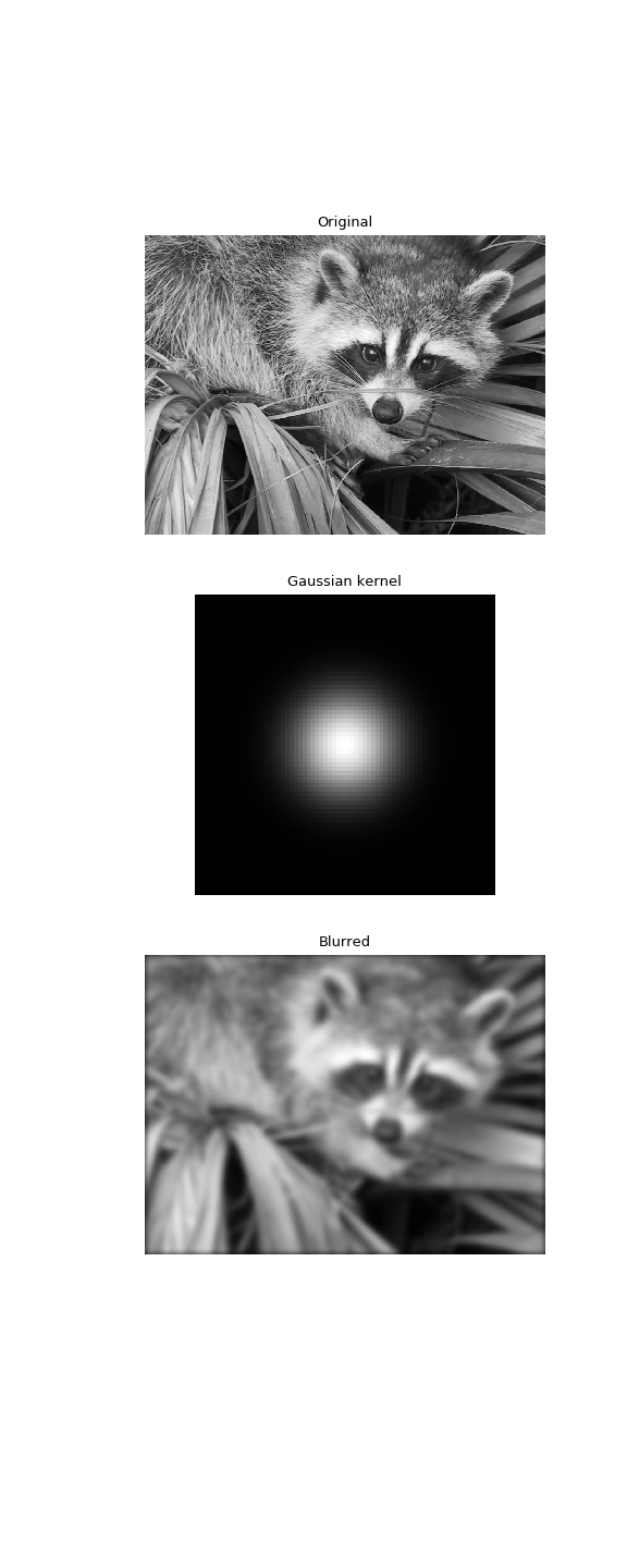
Gaussian blur implemented using FFT convolution. Notice the dark borders around the image, due to the zero-padding beyond its boundaries. The
convolve2dfunction allows for other types of image boundaries, but is far slower.>>> from scipy import misc >>> face = misc.face(gray=True) >>> kernel = np.outer(signal.gaussian(70, 8), signal.gaussian(70, 8)) >>> blurred = signal.fftconvolve(face, kernel, mode='same')
>>> fig, (ax_orig, ax_kernel, ax_blurred) = plt.subplots(3, 1,
...                                                      figsize=(6, 15))
>>> ax_orig.imshow(face, cmap='gray')
>>> ax_orig.set_title('Original')
>>> ax_orig.set_axis_off()
>>> ax_kernel.imshow(kernel, cmap='gray')
>>> ax_kernel.set_title('Gaussian kernel')
>>> ax_kernel.set_axis_off()
>>> ax_blurred.imshow(blurred, cmap='gray')
>>> ax_blurred.set_title('Blurred')
>>> ax_blurred.set_axis_off()
>>> fig.show()