scipy.stats.poisson
-
scipy.stats.poisson= <scipy.stats._discrete_distns.poisson_gen object>[source]¶ A Poisson discrete random variable.
As an instance of the
rv_discreteclass,poissonobject inherits from it a collection of generic methods (see below for the full list), and completes them with details specific for this particular distribution.Notes
The probability mass function for
poissonis:\[f(k) = \exp(-\mu) \frac{\mu^k}{k!}\]for \(k \ge 0\).
poissontakes \(\mu\) as shape parameter.The probability mass function above is defined in the “standardized” form. To shift distribution use the
locparameter. Specifically,poisson.pmf(k, mu, loc)is identically equivalent topoisson.pmf(k - loc, mu).Examples
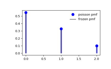
>>> from scipy.stats import poisson
>>> import matplotlib.pyplot as plt
>>> fig, ax = plt.subplots(1, 1)
Calculate a few first moments:
>>> mu = 0.6
>>> mean, var, skew, kurt = poisson.stats(mu, moments='mvsk')
Display the probability mass function (
pmf):>>> x = np.arange(poisson.ppf(0.01, mu), ... poisson.ppf(0.99, mu)) >>> ax.plot(x, poisson.pmf(x, mu), 'bo', ms=8, label='poisson pmf') >>> ax.vlines(x, 0, poisson.pmf(x, mu), colors='b', lw=5, alpha=0.5)
Alternatively, the distribution object can be called (as a function) to fix the shape and location. This returns a “frozen” RV object holding the given parameters fixed.
Freeze the distribution and display the frozen
pmf:>>> rv = poisson(mu) >>> ax.vlines(x, 0, rv.pmf(x), colors='k', linestyles='-', lw=1, ... label='frozen pmf') >>> ax.legend(loc='best', frameon=False) >>> plt.show()
Check accuracy of
cdfandppf:>>> prob = poisson.cdf(x, mu) >>> np.allclose(x, poisson.ppf(prob, mu)) True
Generate random numbers:
>>> r = poisson.rvs(mu, size=1000)
Methods
rvs(mu, loc=0, size=1, random_state=None)
Random variates.
pmf(k, mu, loc=0)
Probability mass function.
logpmf(k, mu, loc=0)
Log of the probability mass function.
cdf(k, mu, loc=0)
Cumulative distribution function.
logcdf(k, mu, loc=0)
Log of the cumulative distribution function.
sf(k, mu, loc=0)
Survival function (also defined as
1 - cdf, but sf is sometimes more accurate).logsf(k, mu, loc=0)
Log of the survival function.
ppf(q, mu, loc=0)
Percent point function (inverse of
cdf— percentiles).isf(q, mu, loc=0)
Inverse survival function (inverse of
sf).stats(mu, loc=0, moments=’mv’)
Mean(‘m’), variance(‘v’), skew(‘s’), and/or kurtosis(‘k’).
entropy(mu, loc=0)
(Differential) entropy of the RV.
expect(func, args=(mu,), loc=0, lb=None, ub=None, conditional=False)
Expected value of a function (of one argument) with respect to the distribution.
median(mu, loc=0)
Median of the distribution.
mean(mu, loc=0)
Mean of the distribution.
var(mu, loc=0)
Variance of the distribution.
std(mu, loc=0)
Standard deviation of the distribution.
interval(alpha, mu, loc=0)
Endpoints of the range that contains alpha percent of the distribution