scipy.spatial.SphericalVoronoi
-
class
scipy.spatial.SphericalVoronoi(points, radius=None, center=None, threshold=1e-06)[source]¶ Voronoi diagrams on the surface of a sphere.
New in version 0.18.0.
- Parameters
- pointsndarray of floats, shape (npoints, 3)
Coordinates of points to construct a spherical Voronoi diagram from
- radiusfloat, optional
Radius of the sphere (Default: 1)
- centerndarray of floats, shape (3,)
Center of sphere (Default: origin)
- thresholdfloat
Threshold for detecting duplicate points and mismatches between points and sphere parameters. (Default: 1e-06)
- Raises
- ValueError
If there are duplicates in points. If the provided radius is not consistent with points.
See also
VoronoiConventional Voronoi diagrams in N dimensions.
Notes
The spherical Voronoi diagram algorithm proceeds as follows. The Convex Hull of the input points (generators) is calculated, and is equivalent to their Delaunay triangulation on the surface of the sphere [R9133a064969a-Caroli]. A 3D Delaunay tetrahedralization is obtained by including the origin of the coordinate system as the fourth vertex of each simplex of the Convex Hull. The circumcenters of all tetrahedra in the system are calculated and projected to the surface of the sphere, producing the Voronoi vertices. The Delaunay tetrahedralization neighbour information is then used to order the Voronoi region vertices around each generator. The latter approach is substantially less sensitive to floating point issues than angle-based methods of Voronoi region vertex sorting.
The surface area of spherical polygons is calculated by decomposing them into triangles and using L’Huilier’s Theorem to calculate the spherical excess of each triangle [R9133a064969a-Weisstein]. The sum of the spherical excesses is multiplied by the square of the sphere radius to obtain the surface area of the spherical polygon. For nearly-degenerate spherical polygons an area of approximately 0 is returned by default, rather than attempting the unstable calculation.
Empirical assessment of spherical Voronoi algorithm performance suggests quadratic time complexity (loglinear is optimal, but algorithms are more challenging to implement). The reconstitution of the surface area of the sphere, measured as the sum of the surface areas of all Voronoi regions, is closest to 100 % for larger (>> 10) numbers of generators.
References
- R9133a064969a-Caroli
Caroli et al. Robust and Efficient Delaunay triangulations of points on or close to a sphere. Research Report RR-7004, 2009.
- R9133a064969a-Weisstein
“L’Huilier’s Theorem.” From MathWorld – A Wolfram Web Resource. http://mathworld.wolfram.com/LHuiliersTheorem.html
Examples
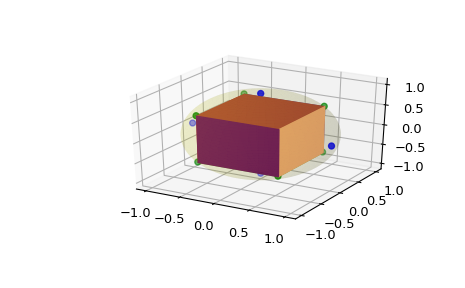
>>> from matplotlib import colors
>>> from mpl_toolkits.mplot3d.art3d import Poly3DCollection
>>> import matplotlib.pyplot as plt
>>> from scipy.spatial import SphericalVoronoi
>>> from mpl_toolkits.mplot3d import proj3d
>>> # set input data
>>> points = np.array([[0, 0, 1], [0, 0, -1], [1, 0, 0],
...                    [0, 1, 0], [0, -1, 0], [-1, 0, 0], ])
>>> center = np.array([0, 0, 0])
>>> radius = 1
>>> # calculate spherical Voronoi diagram
>>> sv = SphericalVoronoi(points, radius, center)
>>> # sort vertices (optional, helpful for plotting)
>>> sv.sort_vertices_of_regions()
>>> # generate plot
>>> fig = plt.figure()
>>> ax = fig.add_subplot(111, projection='3d')
>>> # plot the unit sphere for reference (optional)
>>> u = np.linspace(0, 2 * np.pi, 100)
>>> v = np.linspace(0, np.pi, 100)
>>> x = np.outer(np.cos(u), np.sin(v))
>>> y = np.outer(np.sin(u), np.sin(v))
>>> z = np.outer(np.ones(np.size(u)), np.cos(v))
>>> ax.plot_surface(x, y, z, color='y', alpha=0.1)
>>> # plot generator points
>>> ax.scatter(points[:, 0], points[:, 1], points[:, 2], c='b')
>>> # plot Voronoi vertices
>>> ax.scatter(sv.vertices[:, 0], sv.vertices[:, 1], sv.vertices[:, 2],
...                    c='g')
>>> # indicate Voronoi regions (as Euclidean polygons)
>>> for region in sv.regions:
...    random_color = colors.rgb2hex(np.random.rand(3))
...    polygon = Poly3DCollection([sv.vertices[region]], alpha=1.0)
...    polygon.set_color(random_color)
...    ax.add_collection3d(polygon)
>>> plt.show()
- Attributes
- pointsdouble array of shape (npoints, 3)
the points in 3D to generate the Voronoi diagram from
- radiusdouble
radius of the sphere Default: None (forces estimation, which is less precise)
- centerdouble array of shape (3,)
center of the sphere Default: None (assumes sphere is centered at origin)
- verticesdouble array of shape (nvertices, 3)
Voronoi vertices corresponding to points
- regionslist of list of integers of shape (npoints, _ )
the n-th entry is a list consisting of the indices of the vertices belonging to the n-th point in points
Methods
sort_vertices_of_regions(self)For each region in regions, it sorts the indices of the Voronoi vertices such that the resulting points are in a clockwise or counterclockwise order around the generator point.