scipy.signal.windows.hamming

scipy.signal.windows.hamming(M, sym=True)

Return a Hamming window.

The Hamming window is a taper formed by using a raised cosine with non-zero endpoints, optimized to minimize the nearest side lobe.

Parameters:

M : int

Number of points in the output window. If zero or less, an empty array is returned.

sym : bool, optional

When True (default), generates a symmetric window, for use in filter design. When False, generates a periodic window, for use in spectral analysis.

Returns:

w : ndarray

The window, with the maximum value normalized to 1 (though the value 1 does not appear if M is even and sym is True).

Notes

The Hamming window is defined as

\[w(n) = 0.54 - 0.46 \cos\left(\frac{2\pi{n}}{M-1}\right) \qquad 0 \leq n \leq M-1\]

The Hamming was named for R. W. Hamming, an associate of J. W. Tukey and is described in Blackman and Tukey. It was recommended for smoothing the truncated autocovariance function in the time domain. Most references to the Hamming window come from the signal processing literature, where it is used as one of many windowing functions for smoothing values. It is also known as an apodization (which means “removing the foot”, i.e. smoothing discontinuities at the beginning and end of the sampled signal) or tapering function.

References

[1]	Blackman, R.B. and Tukey, J.W., (1958) The measurement of power spectra, Dover Publications, New York.

[2]	E.R. Kanasewich, “Time Sequence Analysis in Geophysics”, The University of Alberta Press, 1975, pp. 109-110.

[3]	Wikipedia, “Window function”, https://en.wikipedia.org/wiki/Window_function

[4]	W.H. Press, B.P. Flannery, S.A. Teukolsky, and W.T. Vetterling, “Numerical Recipes”, Cambridge University Press, 1986, page 425.

Examples

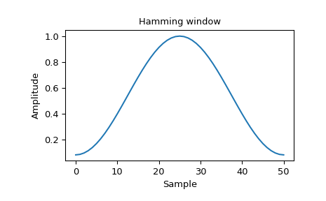
Plot the window and its frequency response:

>>> from scipy import signal
>>> from scipy.fftpack import fft, fftshift
>>> import matplotlib.pyplot as plt

>>> window = signal.hamming(51)
>>> plt.plot(window)
>>> plt.title("Hamming window")
>>> plt.ylabel("Amplitude")
>>> plt.xlabel("Sample")

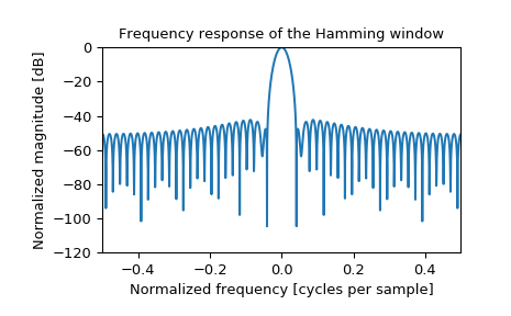
>>> plt.figure()
>>> A = fft(window, 2048) / (len(window)/2.0)
>>> freq = np.linspace(-0.5, 0.5, len(A))
>>> response = 20 * np.log10(np.abs(fftshift(A / abs(A).max())))
>>> plt.plot(freq, response)
>>> plt.axis([-0.5, 0.5, -120, 0])
>>> plt.title("Frequency response of the Hamming window")
>>> plt.ylabel("Normalized magnitude [dB]")
>>> plt.xlabel("Normalized frequency [cycles per sample]")