scipy.signal.freqz

scipy.signal.freqz(b, a=1, worN=512, whole=False, plot=None, fs=6.283185307179586)

Compute the frequency response of a digital filter.

Given the M-order numerator b and N-order denominator a of a digital filter, compute its frequency response:

            jw                 -jw              -jwM
   jw    B(e  )    b[0] + b[1]e    + ... + b[M]e
H(e  ) = ------ = -----------------------------------
            jw                 -jw              -jwN
         A(e  )    a[0] + a[1]e    + ... + a[N]e

Parameters:

b : array_like

Numerator of a linear filter. If b has dimension greater than 1, it is assumed that the coefficients are stored in the first dimension, and b.shape[1:], a.shape[1:], and the shape of the frequencies array must be compatible for broadcasting.

a : array_like

Denominator of a linear filter. If b has dimension greater than 1, it is assumed that the coefficients are stored in the first dimension, and b.shape[1:], a.shape[1:], and the shape of the frequencies array must be compatible for broadcasting.

worN : {None, int, array_like}, optional

If a single integer, then compute at that many frequencies (default is N=512). This is a convenient alternative to:

np.linspace(0, fs if whole else fs/2, N, endpoint=False)

Using a number that is fast for FFT computations can result in faster computations (see Notes).

If an array_like, compute the response at the frequencies given. These are in the same units as fs.

whole : bool, optional

Normally, frequencies are computed from 0 to the Nyquist frequency, fs/2 (upper-half of unit-circle). If whole is True, compute frequencies from 0 to fs. Ignored if w is array_like.

plot : callable

A callable that takes two arguments. If given, the return parameters w and h are passed to plot. Useful for plotting the frequency response inside freqz.

fs : float, optional

The sampling frequency of the digital system. Defaults to 2*pi radians/sample (so w is from 0 to pi).

New in version 1.2.0.

Returns:

w : ndarray

The frequencies at which h was computed, in the same units as fs. By default, w is normalized to the range [0, pi) (radians/sample).

h : ndarray

The frequency response, as complex numbers.

See also

freqz_zpk, sosfreqz

Notes

Using Matplotlib’s matplotlib.pyplot.plot function as the callable for plot produces unexpected results, as this plots the real part of the complex transfer function, not the magnitude. Try lambda w, h: plot(w, np.abs(h)).

A direct computation via (R)FFT is used to compute the frequency response when the following conditions are met:

1. An integer value is given for worN.
2. worN is fast to compute via FFT (i.e., next_fast_len(worN) equals worN).
3. The denominator coefficients are a single value (a.shape[0] == 1).
4. worN is at least as long as the numerator coefficients (worN >= b.shape[0]).
5. If b.ndim > 1, then b.shape[-1] == 1.

For long FIR filters, the FFT approach can have lower error and be much faster than the equivalent direct polynomial calculation.

Examples

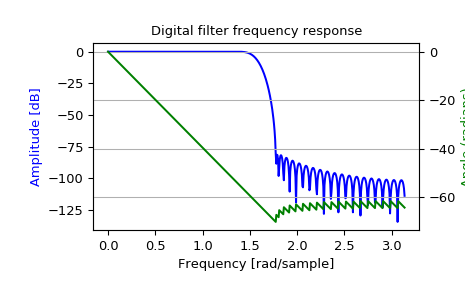
>>> from scipy import signal
>>> b = signal.firwin(80, 0.5, window=('kaiser', 8))
>>> w, h = signal.freqz(b)

>>> import matplotlib.pyplot as plt
>>> fig, ax1 = plt.subplots()
>>> ax1.set_title('Digital filter frequency response')

>>> ax1.plot(w, 20 * np.log10(abs(h)), 'b')
>>> ax1.set_ylabel('Amplitude [dB]', color='b')
>>> ax1.set_xlabel('Frequency [rad/sample]')

>>> ax2 = ax1.twinx()
>>> angles = np.unwrap(np.angle(h))
>>> ax2.plot(w, angles, 'g')
>>> ax2.set_ylabel('Angle (radians)', color='g')
>>> ax2.grid()
>>> ax2.axis('tight')
>>> plt.show()

Broadcasting Examples

Suppose we have two FIR filters whose coefficients are stored in the rows of an array with shape (2, 25). For this demonstration we’ll use random data:

>>> np.random.seed(42)
>>> b = np.random.rand(2, 25)

To compute the frequency response for these two filters with one call to freqz, we must pass in b.T, because freqz expects the first axis to hold the coefficients. We must then extend the shape with a trivial dimension of length 1 to allow broadcasting with the array of frequencies. That is, we pass in b.T[..., np.newaxis], which has shape (25, 2, 1):

>>> w, h = signal.freqz(b.T[..., np.newaxis], worN=1024)
>>> w.shape
(1024,)
>>> h.shape
(2, 1024)

Now suppose we have two transfer functions, with the same numerator coefficients b = [0.5, 0.5]. The coefficients for the two denominators are stored in the first dimension of the two-dimensional array a:

a = [   1      1  ]
    [ -0.25, -0.5 ]

>>> b = np.array([0.5, 0.5])
>>> a = np.array([[1, 1], [-0.25, -0.5]])

Only a is more than one-dimensional. To make it compatible for broadcasting with the frequencies, we extend it with a trivial dimension in the call to freqz:

>>> w, h = signal.freqz(b, a[..., np.newaxis], worN=1024)
>>> w.shape
(1024,)
>>> h.shape
(2, 1024)