scipy.special.stdtrit#
- scipy.special.stdtrit(df, p, out=None) = <ufunc 'stdtrit'>#
The p-th quantile of the student t distribution.
This function is the inverse of the student t distribution cumulative distribution function (CDF), returning t such that stdtr(df, t) = p.
Returns the argument t such that stdtr(df, t) is equal to p.
- Parameters:
- dfarray_like
Degrees of freedom
- parray_like
Probability
- outndarray, optional
Optional output array for the function results
- Returns:
- tscalar or ndarray
Value of t such that
stdtr(df, t) == p
See also
stdtrStudent t CDF
stdtridfinverse of stdtr with respect to df
scipy.stats.tStudent t distribution
Notes
The student t distribution is also available as
scipy.stats.t. Callingstdtritdirectly can improve performance compared to theppfmethod ofscipy.stats.t(see last example below).stdtrithas experimental support for Python Array API Standard compatible backends in addition to NumPy. Please consider testing these features by setting an environment variableSCIPY_ARRAY_API=1and providing CuPy, PyTorch, JAX, or Dask arrays as array arguments. The following combinations of backend and device (or other capability) are supported.Library
CPU
GPU
NumPy
✅
n/a
CuPy
n/a
✅
PyTorch
✅
⛔
JAX
⛔
⛔
Dask
✅
n/a
See Support for the array API standard for more information.
Examples
stdtritrepresents the inverse of the student t distribution CDF which is available asstdtr. Here, we calculate the CDF fordfatx=1.stdtritthen returns1up to floating point errors given the same value for df and the computed CDF value.>>> import numpy as np >>> from scipy.special import stdtr, stdtrit >>> import matplotlib.pyplot as plt >>> df = 3 >>> x = 1 >>> cdf_value = stdtr(df, x) >>> stdtrit(df, cdf_value) 0.9999999994418539
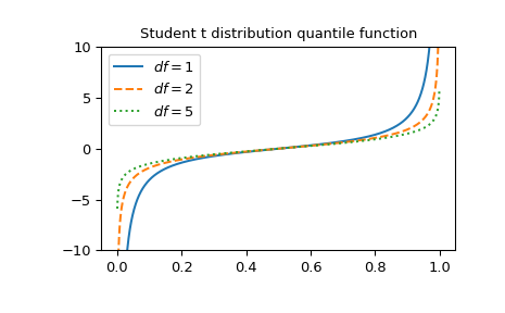
Plot the function for three different degrees of freedom.
>>> x = np.linspace(0, 1, 1000)
>>> parameters = [(1, "solid"), (2, "dashed"), (5, "dotted")]
>>> fig, ax = plt.subplots()
>>> for (df, linestyle) in parameters:
...     ax.plot(x, stdtrit(df, x), ls=linestyle, label=f"$df={df}$")
>>> ax.legend()
>>> ax.set_ylim(-10, 10)
>>> ax.set_title("Student t distribution quantile function")
>>> plt.show()
The function can be computed for several degrees of freedom at the same time by providing a NumPy array or list for df:
>>> stdtrit([1, 2, 3], 0.7)
array([0.72654253, 0.6172134 , 0.58438973])
It is possible to calculate the function at several points for several different degrees of freedom simultaneously by providing arrays for df and p with shapes compatible for broadcasting. Compute
stdtritat 4 points for 3 degrees of freedom resulting in an array of shape 3x4.>>> dfs = np.array([[1], [2], [3]]) >>> p = np.array([0.2, 0.4, 0.7, 0.8]) >>> dfs.shape, p.shape ((3, 1), (4,))
>>> stdtrit(dfs, p)
array([[-1.37638192, -0.3249197 ,  0.72654253,  1.37638192],
       [-1.06066017, -0.28867513,  0.6172134 ,  1.06066017],
       [-0.97847231, -0.27667066,  0.58438973,  0.97847231]])
The t distribution is also available as
scipy.stats.t. Callingstdtritdirectly can be much faster than calling theppfmethod ofscipy.stats.t. To get the same results, one must use the following parametrization:scipy.stats.t(df).ppf(x) = stdtrit(df, x).>>> from scipy.stats import t >>> df, x = 3, 0.5 >>> stdtrit_result = stdtrit(df, x) # this can be faster than below >>> stats_result = t(df).ppf(x) >>> stats_result == stdtrit_result # test that results are equal True