scipy.special.fdtr#
- scipy.special.fdtr(dfn, dfd, x, out=None) = <ufunc 'fdtr'>#
F cumulative distribution function.
Returns the value of the cumulative distribution function of the F-distribution, also known as Snedecor’s F-distribution or the Fisher-Snedecor distribution.
The F-distribution with parameters \(d_n\) and \(d_d\) is the distribution of the random variable,
\[X = \frac{U_n/d_n}{U_d/d_d},\]where \(U_n\) and \(U_d\) are random variables distributed \(\chi^2\), with \(d_n\) and \(d_d\) degrees of freedom, respectively.
- Parameters:
- dfnarray_like
First parameter (positive float).
- dfdarray_like
Second parameter (positive float).
- xarray_like
Argument (nonnegative float).
- outndarray, optional
Optional output array for the function values
- Returns:
- yscalar or ndarray
The CDF of the F-distribution with parameters dfn and dfd at x.
See also
fdtrcF distribution survival function
fdtriF distribution inverse cumulative distribution
scipy.stats.fF distribution
Notes
The regularized incomplete beta function is used, according to the formula,
\[F(d_n, d_d; x) = I_{xd_n/(d_d + xd_n)}(d_n/2, d_d/2).\]Wrapper for the Cephes [1] routine
fdtr. The F distribution is also available asscipy.stats.f. Callingfdtrdirectly can improve performance compared to thecdfmethod ofscipy.stats.f(see last example below).References
[1]Cephes Mathematical Functions Library, http://www.netlib.org/cephes/
Examples
Calculate the function for
dfn=1anddfd=2atx=1.>>> import numpy as np >>> from scipy.special import fdtr >>> fdtr(1, 2, 1) 0.5773502691896258
Calculate the function at several points by providing a NumPy array for x.
>>> x = np.array([0.5, 2., 3.])
>>> fdtr(1, 2, x)
array([0.4472136 , 0.70710678, 0.77459667])
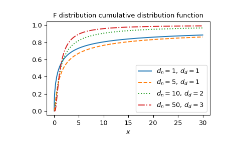
Plot the function for several parameter sets.
>>> import matplotlib.pyplot as plt
>>> dfn_parameters = [1, 5, 10, 50]
>>> dfd_parameters = [1, 1, 2, 3]
>>> linestyles = ['solid', 'dashed', 'dotted', 'dashdot']
>>> parameters_list = list(zip(dfn_parameters, dfd_parameters,
...                            linestyles))
>>> x = np.linspace(0, 30, 1000)
>>> fig, ax = plt.subplots()
>>> for parameter_set in parameters_list:
...     dfn, dfd, style = parameter_set
...     fdtr_vals = fdtr(dfn, dfd, x)
...     ax.plot(x, fdtr_vals, label=rf"$d_n={dfn},\, d_d={dfd}$",
...             ls=style)
>>> ax.legend()
>>> ax.set_xlabel("$x$")
>>> ax.set_title("F distribution cumulative distribution function")
>>> plt.show()
The F distribution is also available as
scipy.stats.f. Usingfdtrdirectly can be much faster than calling thecdfmethod ofscipy.stats.f, especially for small arrays or individual values. To get the same results one must use the following parametrization:stats.f(dfn, dfd).cdf(x)=fdtr(dfn, dfd, x).>>> from scipy.stats import f >>> dfn, dfd = 1, 2 >>> x = 1 >>> fdtr_res = fdtr(dfn, dfd, x) # this will often be faster than below >>> f_dist_res = f(dfn, dfd).cdf(x) >>> fdtr_res == f_dist_res # test that results are equal True