Normal#
- class scipy.stats.Normal(mu=None, sigma=None, **kwargs)[source]#
Normal distribution with prescribed mean and standard deviation.
The probability density function of the normal distribution is:
\[f(x) = \frac{1}{\sigma \sqrt{2 \pi}} \exp { \left( -\frac{1}{2}\left( \frac{x - \mu}{\sigma} \right)^2 \right)}\]for \(x\) in (-infty, infty). This class accepts one parameterization:
mufor \(\mu \in (-\infty, \infty)\),sigmafor \(\sigma \in (0, \infty)\).- Parameters:
- tolpositive float, optional
The desired relative tolerance of calculations. Left unspecified, calculations may be faster; when provided, calculations may be more likely to meet the desired accuracy.
- validation_policy{None, “skip_all”}
Specifies the level of input validation to perform. Left unspecified, input validation is performed to ensure appropriate behavior in edge case (e.g. parameters out of domain, argument outside of distribution support, etc.) and improve consistency of output dtype, shape, etc. Pass
'skip_all'to avoid the computational overhead of these checks when rough edges are acceptable.- cache_policy{None, “no_cache”}
Specifies the extent to which intermediate results are cached. Left unspecified, intermediate results of some calculations (e.g. distribution support, moments, etc.) are cached to improve performance of future calculations. Pass
'no_cache'to reduce memory reserved by the class instance.
See also
- Random Variable Transition Guide
Tutorial
Notes
The following abbreviations are used throughout the documentation.
PDF: probability density function
CDF: cumulative distribution function
CCDF: complementary CDF
entropy: differential entropy
log-F: logarithm of F (e.g. log-CDF)
inverse F: inverse function of F (e.g. inverse CDF)
The API documentation is written to describe the API, not to serve as a statistical reference. Effort is made to be correct at the level required to use the functionality, not to be mathematically rigorous. For example, continuity and differentiability may be implicitly assumed. For precise mathematical definitions, consult your preferred mathematical text.
Examples
To use the distribution class, it must be instantiated using keyword parameters corresponding with one of the accepted parameterizations.
>>> import numpy as np
>>> import matplotlib.pyplot as plt
>>> from scipy import stats
>>> from scipy.stats import Normal
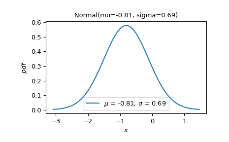
>>> X = Normal(mu=-0.81, sigma=0.69)
For convenience, the
plotmethod can be used to visualize the density and other functions of the distribution.>>> X.plot() >>> plt.show()

The support of the underlying distribution is available using the
supportmethod.>>> X.support() (-inf, inf)
The numerical values of parameters associated with all parameterizations are available as attributes.
>>> X.mu, X.sigma
(-0.81, 0.69)
To evaluate the probability density function of the underlying distribution at argument
x=-1.13:>>> x = -1.13 >>> X.pdf(x) 0.5192263911374636
The cumulative distribution function, its complement, and the logarithm of these functions are evaluated similarly.
>>> np.allclose(np.exp(X.logccdf(x)), 1 - X.cdf(x))
True
The inverse of these functions with respect to the argument
xis also available.>>> logp = np.log(1 - X.ccdf(x)) >>> np.allclose(X.ilogcdf(logp), x) True
Note that distribution functions and their logarithms also have two-argument versions for working with the probability mass between two arguments. The result tends to be more accurate than the naive implementation because it avoids subtractive cancellation.
>>> y = -0.56
>>> np.allclose(X.ccdf(x, y), 1 - (X.cdf(y) - X.cdf(x)))
True
There are methods for computing measures of central tendency, dispersion, higher moments, and entropy.
>>> X.mean(), X.median(), X.mode()
(-0.81, -0.81, -0.81)
>>> X.variance(), X.standard_deviation()
(0.4760999999999999, 0.69)
>>> X.skewness(), X.kurtosis()
(0.0, 3.0)
>>> np.allclose(X.moment(order=6, kind='standardized'),
...             X.moment(order=6, kind='central') / X.variance()**3)
True
>>> np.allclose(np.exp(X.logentropy()), X.entropy())
True
Pseudo-random samples can be drawn from the underlying distribution using
sample.>>> X.sample(shape=(4,)) array([-1.48808956, -0.51999038, -1.29484866, -0.57072244]) # may vary
- Attributes:
- All parameters are available as attributes.
Methods
support()Support of the random variable
plot([x, y, t, ax])Plot a function of the distribution.
sample([shape, method, rng])Random sample from the distribution.
moment([order, kind, method])Raw, central, or standard moment of positive integer order.
mean(*[, method])Mean (raw first moment about the origin)
median(*[, method])Median (50th percentil)
mode(*[, method])Mode (most likely value)
variance(*[, method])Variance (central second moment)
standard_deviation(*[, method])Standard deviation (square root of the second central moment)
skewness(*[, method])Skewness (standardized third moment)
kurtosis(*[, method, convention])Kurtosis (standardized fourth moment)
pdf(x, /, *[, method])Probability density function
logpdf(x, /, *[, method])Log of the probability density function
cdf(x[, y, method])Cumulative distribution function
icdf(p, /, *[, method])Inverse of the cumulative distribution function.
ccdf(x[, y, method])Complementary cumulative distribution function
iccdf(p, /, *[, method])Inverse complementary cumulative distribution function.
logcdf(x[, y, method])Log of the cumulative distribution function
ilogcdf(logp, /, *[, method])Inverse of the logarithm of the cumulative distribution function.
logccdf(x[, y, method])Log of the complementary cumulative distribution function
ilogccdf(logp, /, *[, method])Inverse of the log of the complementary cumulative distribution function.
entropy(*[, method])Differential entropy
logentropy(*[, method])Logarithm of the differential entropy