Akima1DInterpolator#
- class scipy.interpolate.Akima1DInterpolator(x, y, axis=0, *, method='akima', extrapolate=None)[source]#
Akima interpolator
Fit piecewise cubic polynomials, given vectors x and y. The interpolation method by Akima uses a continuously differentiable sub-spline built from piecewise cubic polynomials. The resultant curve passes through the given data points and will appear smooth and natural.
- Parameters:
- xndarray, shape (npoints, )
1-D array of monotonically increasing real values.
- yndarray, shape (…, npoints, …)
N-D array of real values. The length of
yalong the interpolation axis must be equal to the length ofx. Use theaxisparameter to select the interpolation axis.- axisint, optional
Axis in the
yarray corresponding to the x-coordinate values. Defaults toaxis=0.- method{‘akima’, ‘makima’}, optional
If
"makima", use the modified Akima interpolation [2]. Defaults to"akima", use the Akima interpolation [1].Added in version 1.13.0.
- extrapolate{bool, None}, optional
If bool, determines whether to extrapolate to out-of-bounds points based on first and last intervals, or to return NaNs. If None,
extrapolateis set to False.
See also
PchipInterpolatorPCHIP 1-D monotonic cubic interpolator.
CubicSplineCubic spline data interpolator.
PPolyPiecewise polynomial in terms of coefficients and breakpoints
Notes
Added in version 0.14.
Use only for precise data, as the fitted curve passes through the given points exactly. This routine is useful for plotting a pleasingly smooth curve through a few given points for purposes of plotting.
Let \(\delta_i = (y_{i+1} - y_i) / (x_{i+1} - x_i)\) be the slopes of the interval \(\left[x_i, x_{i+1}\right)\). Akima’s derivative at \(x_i\) is defined as:
\[d_i = \frac{w_1}{w_1 + w_2}\delta_{i-1} + \frac{w_2}{w_1 + w_2}\delta_i\]In the Akima interpolation [1] (
method="akima"), the weights are:\[\begin{split}\begin{aligned} w_1 &= |\delta_{i+1} - \delta_i| \\ w_2 &= |\delta_{i-1} - \delta_{i-2}| \end{aligned}\end{split}\]In the modified Akima interpolation [2] (
method="makima"), to eliminate overshoot and avoid edge cases of both numerator and denominator being equal to 0, the weights are modified as follows:\[\begin{split}\begin{align*} w_1 &= |\delta_{i+1} - \delta_i| + |\delta_{i+1} + \delta_i| / 2 \\ w_2 &= |\delta_{i-1} - \delta_{i-2}| + |\delta_{i-1} + \delta_{i-2}| / 2 \end{align*}\end{split}\]References
[1] (1,2)A new method of interpolation and smooth curve fitting based on local procedures. Hiroshi Akima, J. ACM, October 1970, 17(4), 589-602. DOI:10.1145/321607.321609
[2] (1,2)Makima Piecewise Cubic Interpolation. Cleve Moler and Cosmin Ionita, 2019. https://blogs.mathworks.com/cleve/2019/04/29/makima-piecewise-cubic-interpolation/
Examples
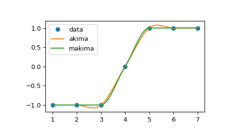
Comparison of
method="akima"andmethod="makima":>>> import numpy as np >>> from scipy.interpolate import Akima1DInterpolator >>> import matplotlib.pyplot as plt >>> x = np.linspace(1, 7, 7) >>> y = np.array([-1, -1, -1, 0, 1, 1, 1]) >>> xs = np.linspace(min(x), max(x), num=100) >>> y_akima = Akima1DInterpolator(x, y, method="akima")(xs) >>> y_makima = Akima1DInterpolator(x, y, method="makima")(xs)
>>> fig, ax = plt.subplots()
>>> ax.plot(x, y, "o", label="data")
>>> ax.plot(xs, y_akima, label="akima")
>>> ax.plot(xs, y_makima, label="makima")
>>> ax.legend()
>>> fig.show()
The overshoot that occurred in
"akima"has been avoided in"makima".
- Attributes:
- axis
- c
- extrapolate
- x
Methods
__call__(x[, nu, extrapolate])Evaluate the piecewise polynomial or its derivative.
derivative([nu])Construct a new piecewise polynomial representing the derivative.
antiderivative([nu])Construct a new piecewise polynomial representing the antiderivative.
roots([discontinuity, extrapolate])Find real roots of the piecewise polynomial.