scipy.stats.

bootstrap

scipy.stats.bootstrap(data, statistic, *, n_resamples=9999, batch=None, vectorized=None, paired=False, axis=0, confidence_level=0.95, alternative='two-sided', method='BCa', bootstrap_result=None, random_state=None)

Compute a two-sided bootstrap confidence interval of a statistic.

When method is 'percentile' and alternative is 'two-sided', a bootstrap confidence interval is computed according to the following procedure.

1. Resample the data: for each sample in data and for each of n_resamples, take a random sample of the original sample (with replacement) of the same size as the original sample.

2. Compute the bootstrap distribution of the statistic: for each set of resamples, compute the test statistic.

3. Determine the confidence interval: find the interval of the bootstrap distribution that is

   • symmetric about the median and

   • contains confidence_level of the resampled statistic values.

While the 'percentile' method is the most intuitive, it is rarely used in practice. Two more common methods are available, 'basic' (‘reverse percentile’) and 'BCa' (‘bias-corrected and accelerated’); they differ in how step 3 is performed.

If the samples in data are taken at random from their respective distributions \(n\) times, the confidence interval returned by bootstrap will contain the true value of the statistic for those distributions approximately confidence_level\(\, \times \, n\) times.

Parameters:

datasequence of array-like

Each element of data is a sample containing scalar observations from an underlying distribution. Elements of data must be broadcastable to the same shape (with the possible exception of the dimension specified by axis).

Changed in version 1.14.0: bootstrap will now emit a FutureWarning if the shapes of the elements of data are not the same (with the exception of the dimension specified by axis). Beginning in SciPy 1.16.0, bootstrap will explicitly broadcast the elements to the same shape (except along axis) before performing the calculation.

statisticcallable

Statistic for which the confidence interval is to be calculated. statistic must be a callable that accepts len(data) samples as separate arguments and returns the resulting statistic. If vectorized is set True, statistic must also accept a keyword argument axis and be vectorized to compute the statistic along the provided axis.

n_resamplesint, default: 9999

The number of resamples performed to form the bootstrap distribution of the statistic.

batchint, optional

The number of resamples to process in each vectorized call to statistic. Memory usage is O( batch * n ), where n is the sample size. Default is None, in which case batch = n_resamples (or batch = max(n_resamples, n) for method='BCa').

vectorizedbool, optional

If vectorized is set False, statistic will not be passed keyword argument axis and is expected to calculate the statistic only for 1D samples. If True, statistic will be passed keyword argument axis and is expected to calculate the statistic along axis when passed an ND sample array. If None (default), vectorized will be set True if axis is a parameter of statistic. Use of a vectorized statistic typically reduces computation time.

pairedbool, default: False

Whether the statistic treats corresponding elements of the samples in data as paired.

axisint, default: 0

The axis of the samples in data along which the statistic is calculated.

confidence_levelfloat, default: 0.95

The confidence level of the confidence interval.

alternative{‘two-sided’, ‘less’, ‘greater’}, default: 'two-sided'

Choose 'two-sided' (default) for a two-sided confidence interval, 'less' for a one-sided confidence interval with the lower bound at -np.inf, and 'greater' for a one-sided confidence interval with the upper bound at np.inf. The other bound of the one-sided confidence intervals is the same as that of a two-sided confidence interval with confidence_level twice as far from 1.0; e.g. the upper bound of a 95% 'less' confidence interval is the same as the upper bound of a 90% 'two-sided' confidence interval.

method{‘percentile’, ‘basic’, ‘bca’}, default: 'BCa'

Whether to return the ‘percentile’ bootstrap confidence interval ('percentile'), the ‘basic’ (AKA ‘reverse’) bootstrap confidence interval ('basic'), or the bias-corrected and accelerated bootstrap confidence interval ('BCa').

bootstrap_resultBootstrapResult, optional

Provide the result object returned by a previous call to bootstrap to include the previous bootstrap distribution in the new bootstrap distribution. This can be used, for example, to change confidence_level, change method, or see the effect of performing additional resampling without repeating computations.

random_state{None, int, numpy.random.Generator,

numpy.random.RandomState}, optional

Pseudorandom number generator state used to generate resamples.

If random_state is None (or np.random), the numpy.random.RandomState singleton is used. If random_state is an int, a new RandomState instance is used, seeded with random_state. If random_state is already a Generator or RandomState instance then that instance is used.

Returns:

resBootstrapResult

An object with attributes:

confidence_intervalConfidenceInterval

The bootstrap confidence interval as an instance of collections.namedtuple with attributes low and high.

bootstrap_distributionndarray

The bootstrap distribution, that is, the value of statistic for each resample. The last dimension corresponds with the resamples (e.g. res.bootstrap_distribution.shape[-1] == n_resamples).

standard_errorfloat or ndarray

The bootstrap standard error, that is, the sample standard deviation of the bootstrap distribution.

Warns:

DegenerateDataWarning

Generated when method='BCa' and the bootstrap distribution is degenerate (e.g. all elements are identical).

Notes

Elements of the confidence interval may be NaN for method='BCa' if the bootstrap distribution is degenerate (e.g. all elements are identical). In this case, consider using another method or inspecting data for indications that other analysis may be more appropriate (e.g. all observations are identical).

References

[1]

B. Efron and R. J. Tibshirani, An Introduction to the Bootstrap, Chapman & Hall/CRC, Boca Raton, FL, USA (1993)

[2]

Nathaniel E. Helwig, “Bootstrap Confidence Intervals”, http://users.stat.umn.edu/~helwig/notes/bootci-Notes.pdf

[3]

Bootstrapping (statistics), Wikipedia, https://en.wikipedia.org/wiki/Bootstrapping_%28statistics%29

Examples

Try it in your browser!

Suppose we have sampled data from an unknown distribution.

>>> import numpy as np
>>> rng = np.random.default_rng()
>>> from scipy.stats import norm
>>> dist = norm(loc=2, scale=4)  # our "unknown" distribution
>>> data = dist.rvs(size=100, random_state=rng)

We are interested in the standard deviation of the distribution.

>>> std_true = dist.std()      # the true value of the statistic
>>> print(std_true)
4.0
>>> std_sample = np.std(data)  # the sample statistic
>>> print(std_sample)
3.9460644295563863

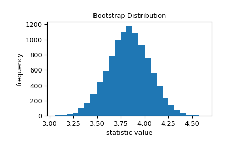
The bootstrap is used to approximate the variability we would expect if we were to repeatedly sample from the unknown distribution and calculate the statistic of the sample each time. It does this by repeatedly resampling values from the original sample with replacement and calculating the statistic of each resample. This results in a “bootstrap distribution” of the statistic.

>>> import matplotlib.pyplot as plt
>>> from scipy.stats import bootstrap
>>> data = (data,)  # samples must be in a sequence
>>> res = bootstrap(data, np.std, confidence_level=0.9,
...                 random_state=rng)
>>> fig, ax = plt.subplots()
>>> ax.hist(res.bootstrap_distribution, bins=25)
>>> ax.set_title('Bootstrap Distribution')
>>> ax.set_xlabel('statistic value')
>>> ax.set_ylabel('frequency')
>>> plt.show()

The standard error quantifies this variability. It is calculated as the standard deviation of the bootstrap distribution.

>>> res.standard_error
0.24427002125829136
>>> res.standard_error == np.std(res.bootstrap_distribution, ddof=1)
True

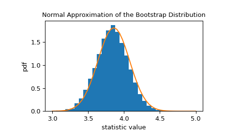
The bootstrap distribution of the statistic is often approximately normal with scale equal to the standard error.

>>> x = np.linspace(3, 5)
>>> pdf = norm.pdf(x, loc=std_sample, scale=res.standard_error)
>>> fig, ax = plt.subplots()
>>> ax.hist(res.bootstrap_distribution, bins=25, density=True)
>>> ax.plot(x, pdf)
>>> ax.set_title('Normal Approximation of the Bootstrap Distribution')
>>> ax.set_xlabel('statistic value')
>>> ax.set_ylabel('pdf')
>>> plt.show()

This suggests that we could construct a 90% confidence interval on the statistic based on quantiles of this normal distribution.

>>> norm.interval(0.9, loc=std_sample, scale=res.standard_error)
(3.5442759991341726, 4.3478528599786)

Due to central limit theorem, this normal approximation is accurate for a variety of statistics and distributions underlying the samples; however, the approximation is not reliable in all cases. Because bootstrap is designed to work with arbitrary underlying distributions and statistics, it uses more advanced techniques to generate an accurate confidence interval.

>>> print(res.confidence_interval)
ConfidenceInterval(low=3.57655333533867, high=4.382043696342881)

If we sample from the original distribution 100 times and form a bootstrap confidence interval for each sample, the confidence interval contains the true value of the statistic approximately 90% of the time.

>>> n_trials = 100
>>> ci_contains_true_std = 0
>>> for i in range(n_trials):
...    data = (dist.rvs(size=100, random_state=rng),)
...    res = bootstrap(data, np.std, confidence_level=0.9,
...                    n_resamples=999, random_state=rng)
...    ci = res.confidence_interval
...    if ci[0] < std_true < ci[1]:
...        ci_contains_true_std += 1
>>> print(ci_contains_true_std)
88

Rather than writing a loop, we can also determine the confidence intervals for all 100 samples at once.

>>> data = (dist.rvs(size=(n_trials, 100), random_state=rng),)
>>> res = bootstrap(data, np.std, axis=-1, confidence_level=0.9,
...                 n_resamples=999, random_state=rng)
>>> ci_l, ci_u = res.confidence_interval

Here, ci_l and ci_u contain the confidence interval for each of the n_trials = 100 samples.

>>> print(ci_l[:5])
[3.86401283 3.33304394 3.52474647 3.54160981 3.80569252]
>>> print(ci_u[:5])
[4.80217409 4.18143252 4.39734707 4.37549713 4.72843584]

And again, approximately 90% contain the true value, std_true = 4.

>>> print(np.sum((ci_l < std_true) & (std_true < ci_u)))
93

bootstrap can also be used to estimate confidence intervals of multi-sample statistics. For example, to get a confidence interval for the difference between means, we write a function that accepts two sample arguments and returns only the statistic. The use of the axis argument ensures that all mean calculations are perform in a single vectorized call, which is faster than looping over pairs of resamples in Python.

>>> def my_statistic(sample1, sample2, axis=-1):
...     mean1 = np.mean(sample1, axis=axis)
...     mean2 = np.mean(sample2, axis=axis)
...     return mean1 - mean2

Here, we use the ‘percentile’ method with the default 95% confidence level.

>>> sample1 = norm.rvs(scale=1, size=100, random_state=rng)
>>> sample2 = norm.rvs(scale=2, size=100, random_state=rng)
>>> data = (sample1, sample2)
>>> res = bootstrap(data, my_statistic, method='basic', random_state=rng)
>>> print(my_statistic(sample1, sample2))
0.16661030792089523
>>> print(res.confidence_interval)
ConfidenceInterval(low=-0.29087973240818693, high=0.6371338699912273)

The bootstrap estimate of the standard error is also available.

>>> print(res.standard_error)
0.238323948262459

Paired-sample statistics work, too. For example, consider the Pearson correlation coefficient.

>>> from scipy.stats import pearsonr
>>> n = 100
>>> x = np.linspace(0, 10, n)
>>> y = x + rng.uniform(size=n)
>>> print(pearsonr(x, y)[0])  # element 0 is the statistic
0.9954306665125647

We wrap pearsonr so that it returns only the statistic, ensuring that we use the axis argument because it is available.

>>> def my_statistic(x, y, axis=-1):
...     return pearsonr(x, y, axis=axis)[0]

We call bootstrap using paired=True.

>>> res = bootstrap((x, y), my_statistic, paired=True, random_state=rng)
>>> print(res.confidence_interval)
ConfidenceInterval(low=0.9941504301315878, high=0.996377412215445)

The result object can be passed back into bootstrap to perform additional resampling:

>>> len(res.bootstrap_distribution)
9999
>>> res = bootstrap((x, y), my_statistic, paired=True,
...                 n_resamples=1000, random_state=rng,
...                 bootstrap_result=res)
>>> len(res.bootstrap_distribution)
10999

or to change the confidence interval options:

>>> res2 = bootstrap((x, y), my_statistic, paired=True,
...                  n_resamples=0, random_state=rng, bootstrap_result=res,
...                  method='percentile', confidence_level=0.9)
>>> np.testing.assert_equal(res2.bootstrap_distribution,
...                         res.bootstrap_distribution)
>>> res.confidence_interval
ConfidenceInterval(low=0.9941574828235082, high=0.9963781698210212)

without repeating computation of the original bootstrap distribution.

Go BackOpen In Tab