scipy.stats.sampling.TransformedDensityRejection

class scipy.stats.sampling.TransformedDensityRejection(dist, *, mode=None, center=None, domain=None, c=-0.5, construction_points=30, use_dars=True, max_squeeze_hat_ratio=0.99, random_state=None)

Transformed Density Rejection (TDR) Method.

TDR is an acceptance/rejection method that uses the concavity of a transformed density to construct hat function and squeezes automatically. Most universal algorithms are very slow compared to algorithms that are specialized to that distribution. Algorithms that are fast have a slow setup and require large tables. The aim of this universal method is to provide an algorithm that is not too slow and needs only a short setup. This method can be applied to univariate and unimodal continuous distributions with T-concave density function. See [1] and [2] for more details.

Parameters:

distobject

An instance of a class with pdf and dpdf methods.

• pdf: PDF of the distribution. The signature of the PDF is expected to be: def pdf(self, x: float) -> float. i.e. the PDF should accept a Python float and return a Python float. It doesn’t need to integrate to 1 i.e. the PDF doesn’t need to be normalized.

• dpdf: Derivative of the PDF w.r.t x (i.e. the variate). Must have the same signature as the PDF.

modefloat, optional

(Exact) Mode of the distribution. Default is None.

centerfloat, optional

Approximate location of the mode or the mean of the distribution. This location provides some information about the main part of the PDF and is used to avoid numerical problems. Default is None.

domainlist or tuple of length 2, optional

The support of the distribution. Default is None. When None:

• If a support method is provided by the distribution object dist, it is used to set the domain of the distribution.

• Otherwise the support is assumed to be \((-\infty, \infty)\).

c{-0.5, 0.}, optional

Set parameter c for the transformation function T. The default is -0.5. The transformation of the PDF must be concave in order to construct the hat function. Such a PDF is called T-concave. Currently the following transformations are supported:

\[\begin{split}c = 0.: T(x) &= \log(x)\\ c = -0.5: T(x) &= \frac{1}{\sqrt{x}} \text{ (Default)}\end{split}\]

construction_pointsint or array_like, optional

If an integer, it defines the number of construction points. If it is array-like, the elements of the array are used as construction points. Default is 30.

use_darsbool, optional

If True, “derandomized adaptive rejection sampling” (DARS) is used in setup. See [1] for the details of the DARS algorithm. Default is True.

max_squeeze_hat_ratiofloat, optional

Set upper bound for the ratio (area below squeeze) / (area below hat). It must be a number between 0 and 1. Default is 0.99.

random_state{None, int, numpy.random.Generator,

numpy.random.RandomState}, optional

A NumPy random number generator or seed for the underlying NumPy random number generator used to generate the stream of uniform random numbers. If random_state is None (or np.random), the numpy.random.RandomState singleton is used. If random_state is an int, a new RandomState instance is used, seeded with random_state. If random_state is already a Generator or RandomState instance then that instance is used.

References

[1] (1,2)

UNU.RAN reference manual, Section 5.3.16, “TDR - Transformed Density Rejection”, http://statmath.wu.ac.at/software/unuran/doc/unuran.html#TDR

[2]

Hörmann, Wolfgang. “A rejection technique for sampling from T-concave distributions.” ACM Transactions on Mathematical Software (TOMS) 21.2 (1995): 182-193

[3]

W.R. Gilks and P. Wild (1992). Adaptive rejection sampling for Gibbs sampling, Applied Statistics 41, pp. 337-348.

Examples

Try it in your browser!

>>> from scipy.stats.sampling import TransformedDensityRejection
>>> import numpy as np

Suppose we have a density:

\[\begin{split}f(x) = \begin{cases} 1 - x^2, & -1 \leq x \leq 1 \\ 0, & \text{otherwise} \end{cases}\end{split}\]

The derivative of this density function is:

\[\begin{split}\frac{df(x)}{dx} = \begin{cases} -2x, & -1 \leq x \leq 1 \\ 0, & \text{otherwise} \end{cases}\end{split}\]

Notice that the PDF doesn’t integrate to 1. As this is a rejection based method, we need not have a normalized PDF. To initialize the generator, we can use:

>>> urng = np.random.default_rng()
>>> class MyDist:
...     def pdf(self, x):
...         return 1-x*x
...     def dpdf(self, x):
...         return -2*x
...
>>> dist = MyDist()
>>> rng = TransformedDensityRejection(dist, domain=(-1, 1),
...                                   random_state=urng)

Domain can be very useful to truncate the distribution but to avoid passing it every time to the constructor, a default domain can be set by providing a support method in the distribution object (dist):

>>> class MyDist:
...     def pdf(self, x):
...         return 1-x*x
...     def dpdf(self, x):
...         return -2*x
...     def support(self):
...         return (-1, 1)
...
>>> dist = MyDist()
>>> rng = TransformedDensityRejection(dist, random_state=urng)

Now, we can use the rvs method to generate samples from the distribution:

>>> rvs = rng.rvs(1000)

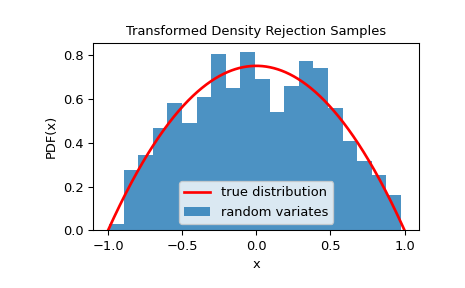
We can check that the samples are from the given distribution by visualizing its histogram:

>>> import matplotlib.pyplot as plt
>>> x = np.linspace(-1, 1, 1000)
>>> fx = 3/4 * dist.pdf(x)  # 3/4 is the normalizing constant
>>> plt.plot(x, fx, 'r-', lw=2, label='true distribution')
>>> plt.hist(rvs, bins=20, density=True, alpha=0.8, label='random variates')
>>> plt.xlabel('x')
>>> plt.ylabel('PDF(x)')
>>> plt.title('Transformed Density Rejection Samples')
>>> plt.legend()
>>> plt.show()

Go BackOpen In Tab

Attributes:

hat_area

Get the area below the hat for the generator.

squeeze_area

Get the area below the squeeze for the generator.

squeeze_hat_ratio

Get the current ratio (area below squeeze) / (area below hat) for the generator.

Methods

ppf_hat(u)	Evaluate the inverse of the CDF of the hat distribution at u.
rvs([size, random_state])	Sample from the distribution.
set_random_state([random_state])	Set the underlying uniform random number generator.