scipy.cluster.hierarchy.linkage#

scipy.cluster.hierarchy.linkage(y, method='single', metric='euclidean', optimal_ordering=False)[source]#

Perform hierarchical/agglomerative clustering.

The input y may be either a 1-D condensed distance matrix or a 2-D array of observation vectors.

If y is a 1-D condensed distance matrix, then y must be a $\binom{n}{2}$ sized vector, where n is the number of original observations paired in the distance matrix. The behavior of this function is very similar to the MATLAB linkage function.

A $(n-1)$ by 4 matrix Z is returned. At the $i$ -th iteration, clusters with indices Z[i, 0] and Z[i, 1] are combined to form cluster $n + i$ . A cluster with an index less than $n$ corresponds to one of the $n$ original observations. The distance between clusters Z[i, 0] and Z[i, 1] is given by Z[i, 2]. The fourth value Z[i, 3] represents the number of original observations in the newly formed cluster.

The following linkage methods are used to compute the distance $d(s, t)$ between two clusters $s$ and $t$ . The algorithm begins with a forest of clusters that have yet to be used in the hierarchy being formed. When two clusters $s$ and $t$ from this forest are combined into a single cluster $u$ , $s$ and $t$ are removed from the forest, and $u$ is added to the forest. When only one cluster remains in the forest, the algorithm stops, and this cluster becomes the root.

A distance matrix is maintained at each iteration. The d[i,j] entry corresponds to the distance between cluster $i$ and $j$ in the original forest.

At each iteration, the algorithm must update the distance matrix to reflect the distance of the newly formed cluster u with the remaining clusters in the forest.

Suppose there are $|u|$ original observations $u[0], \ldots, u[|u|-1]$ in cluster $u$ and $|v|$ original objects $v[0], \ldots, v[|v|-1]$ in cluster $v$ . Recall, $s$ and $t$ are combined to form cluster $u$ . Let $v$ be any remaining cluster in the forest that is not $u$ .

The following are methods for calculating the distance between the newly formed cluster $u$ and each $v$ .

method=’single’ assigns

$d (u, v) = min (d i s t (u [i], v [j]))$
$d(u,v) = \min(dist(u[i],v[j]))$

for all points $i$ in cluster $u$ and $j$ in cluster $v$ . This is also known as the Nearest Point Algorithm.

method=’complete’ assigns

$d (u, v) = max (d i s t (u [i], v [j]))$
$d(u, v) = \max(dist(u[i],v[j]))$

for all points $i$ in cluster u and $j$ in cluster $v$ . This is also known by the Farthest Point Algorithm or Voor Hees Algorithm.

method=’average’ assigns

$d (u, v) = \sum_{i j} \frac{d (u [i], v [j])}{(| u | * | v |)}$
$d(u,v) = \sum_{ij} \frac{d(u[i], v[j])} {(|u|*|v|)}$

for all points $i$ and $j$ where $|u|$ and $|v|$ are the cardinalities of clusters $u$ and $v$ , respectively. This is also called the UPGMA algorithm.

method=’weighted’ assigns

$d (u, v) = (d i s t (s, v) + d i s t (t, v)) / 2$
$d(u,v) = (dist(s,v) + dist(t,v))/2$

where cluster u was formed with cluster s and t and v is a remaining cluster in the forest (also called WPGMA).

method=’centroid’ assigns

$d i s t (s, t) = | | c_{s} - c_{t} | |_{2}$
$dist(s,t) = ||c_s-c_t||_2$

where $c_s$ and $c_t$ are the centroids of clusters $s$ and $t$ , respectively. When two clusters $s$ and $t$ are combined into a new cluster $u$ , the new centroid is computed over all the original objects in clusters $s$ and $t$ . The distance then becomes the Euclidean distance between the centroid of $u$ and the centroid of a remaining cluster $v$ in the forest. This is also known as the UPGMC algorithm.

method=’median’ assigns $d(s,t)$ like the centroid method. When two clusters $s$ and $t$ are combined into a new cluster $u$ , the average of centroids s and t give the new centroid $u$ . This is also known as the WPGMC algorithm.

method=’ward’ uses the Ward variance minimization algorithm. The new entry $d(u,v)$ is computed as follows,

$d (u, v) = \sqrt{\frac{| v | + | s |}{T} d (v, s)^{2} + \frac{| v | + | t |}{T} d (v, t)^{2} - \frac{| v |}{T} d (s, t)^{2}}$
$d(u,v) = \sqrt{\frac{|v|+|s|} {T}d(v,s)^2 + \frac{|v|+|t|} {T}d(v,t)^2 - \frac{|v|} {T}d(s,t)^2}$

where $u$ is the newly joined cluster consisting of clusters $s$ and $t$ , $v$ is an unused cluster in the forest, $T=|v|+|s|+|t|$ , and $|*|$ is the cardinality of its argument. This is also known as the incremental algorithm.

Warning: When the minimum distance pair in the forest is chosen, there may be two or more pairs with the same minimum distance. This implementation may choose a different minimum than the MATLAB version.

Parameters:

yndarray: A condensed distance matrix. A condensed distance matrix is a flat array containing the upper triangular of the distance matrix. This is the form that pdist returns. Alternatively, a collection of $m$ observation vectors in $n$ dimensions may be passed as an $m$ by $n$ array. All elements of the condensed distance matrix must be finite, i.e., no NaNs or infs.
methodstr, optional: The linkage algorithm to use. See the Linkage Methods section below for full descriptions.
metricstr or function, optional: The distance metric to use in the case that y is a collection of observation vectors; ignored otherwise. See the pdist function for a list of valid distance metrics. A custom distance function can also be used.
optimal_orderingbool, optional: If True, the linkage matrix will be reordered so that the distance between successive leaves is minimal. This results in a more intuitive tree structure when the data are visualized. defaults to False, because this algorithm can be slow, particularly on large datasets [2]. See also the optimal_leaf_ordering function.

New in version 1.0.0.

Returns:

Zndarray: The hierarchical clustering encoded as a linkage matrix.

See also

scipy.spatial.distance.pdist: pairwise distance metrics

Notes

For method ‘single’, an optimized algorithm based on minimum spanning tree is implemented. It has time complexity $O(n^2)$ . For methods ‘complete’, ‘average’, ‘weighted’ and ‘ward’, an algorithm called nearest-neighbors chain is implemented. It also has time complexity $O(n^2)$ . For other methods, a naive algorithm is implemented with $O(n^3)$ time complexity. All algorithms use $O(n^2)$ memory. Refer to [1] for details about the algorithms.
Methods ‘centroid’, ‘median’, and ‘ward’ are correctly defined only if Euclidean pairwise metric is used. If y is passed as precomputed pairwise distances, then it is the user’s responsibility to assure that these distances are in fact Euclidean, otherwise the produced result will be incorrect.

References

[1]

Daniel Mullner, “Modern hierarchical, agglomerative clustering algorithms”, arXiv:1109.2378v1.

[2]

Ziv Bar-Joseph, David K. Gifford, Tommi S. Jaakkola, “Fast optimal leaf ordering for hierarchical clustering”, 2001. Bioinformatics DOI:10.1093/bioinformatics/17.suppl_1.S22

Examples

>>> from scipy.cluster.hierarchy import dendrogram, linkage
>>> from matplotlib import pyplot as plt
>>> X = [[i] for i in [2, 8, 0, 4, 1, 9, 9, 0]]

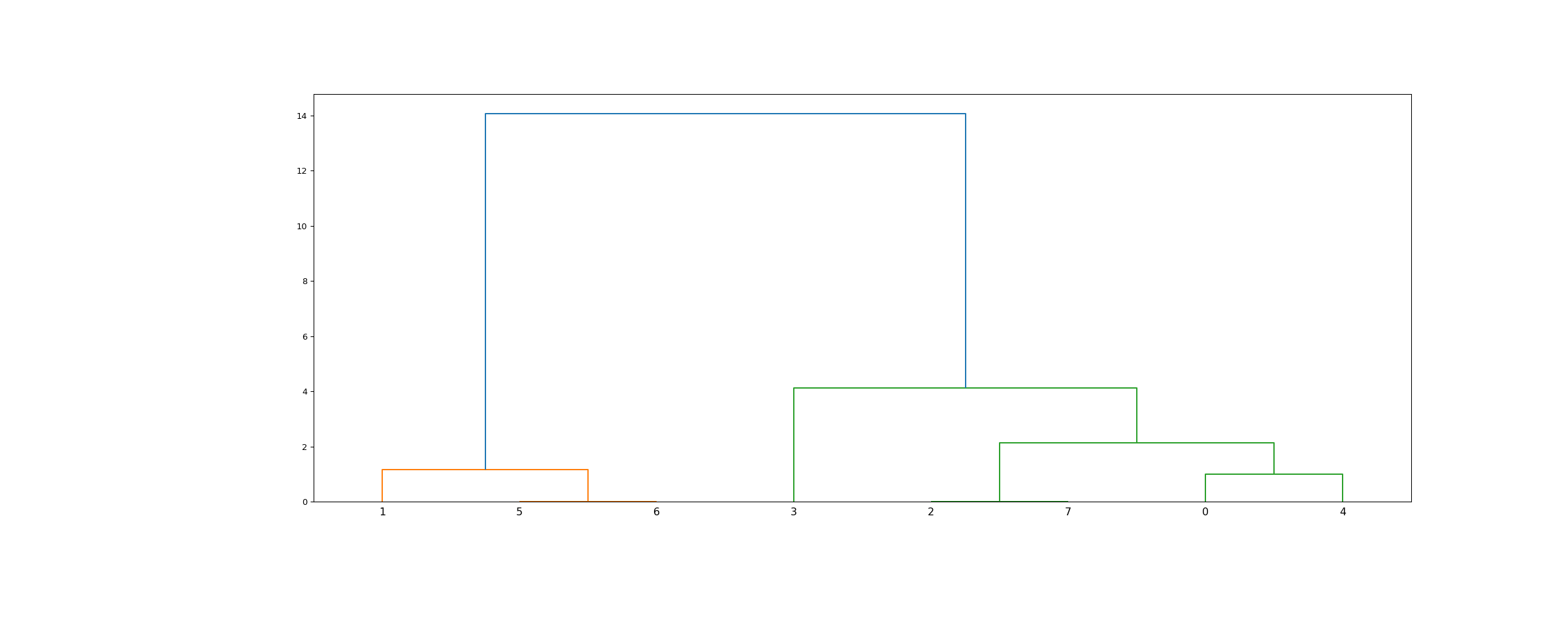
>>> Z = linkage(X, 'ward')
>>> fig = plt.figure(figsize=(25, 10))
>>> dn = dendrogram(Z)

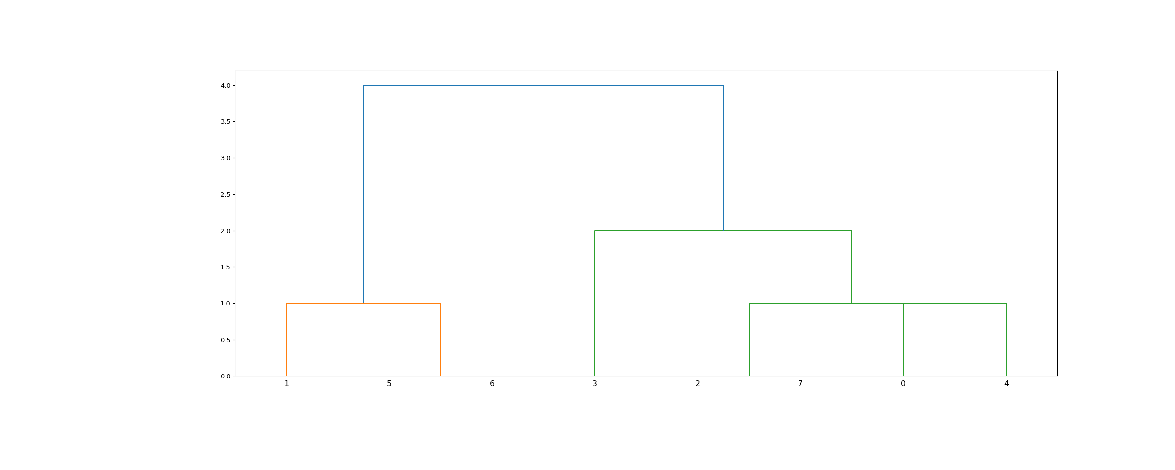
>>> Z = linkage(X, 'single')
>>> fig = plt.figure(figsize=(25, 10))
>>> dn = dendrogram(Z)
>>> plt.show()

../../_images/scipy-cluster-hierarchy-linkage-1_00.png

../../_images/scipy-cluster-hierarchy-linkage-1_01.png