scipy.signal.lsim

scipy.signal.lsim(system, U, T, X0=None, interp=True)

Simulate output of a continuous-time linear system.

Parameters:

systeman instance of the LTI class or a tuple describing the system.

The following gives the number of elements in the tuple and the interpretation:

• 1: (instance of lti)

• 2: (num, den)

• 3: (zeros, poles, gain)

• 4: (A, B, C, D)

Uarray_like

An input array describing the input at each time T (interpolation is assumed between given times). If there are multiple inputs, then each column of the rank-2 array represents an input. If U = 0 or None, a zero input is used.

Tarray_like

The time steps at which the input is defined and at which the output is desired. Must be nonnegative, increasing, and equally spaced.

X0array_like, optional

The initial conditions on the state vector (zero by default).

interpbool, optional

Whether to use linear (True, the default) or zero-order-hold (False) interpolation for the input array.

Returns:

T1D ndarray

Time values for the output.

yout1D ndarray

System response.

xoutndarray

Time evolution of the state vector.

Notes

If (num, den) is passed in for system, coefficients for both the numerator and denominator should be specified in descending exponent order (e.g. s^2 + 3s + 5 would be represented as [1, 3, 5]).

Examples

We’ll use lsim to simulate an analog Bessel filter applied to a signal.

>>> import numpy as np
>>> from scipy.signal import bessel, lsim
>>> import matplotlib.pyplot as plt

Create a low-pass Bessel filter with a cutoff of 12 Hz.

>>> b, a = bessel(N=5, Wn=2*np.pi*12, btype='lowpass', analog=True)

Generate data to which the filter is applied.

>>> t = np.linspace(0, 1.25, 500, endpoint=False)

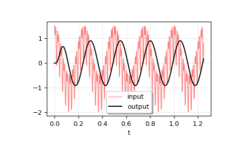
The input signal is the sum of three sinusoidal curves, with frequencies 4 Hz, 40 Hz, and 80 Hz. The filter should mostly eliminate the 40 Hz and 80 Hz components, leaving just the 4 Hz signal.

>>> u = (np.cos(2*np.pi*4*t) + 0.6*np.sin(2*np.pi*40*t) +
...      0.5*np.cos(2*np.pi*80*t))

Simulate the filter with lsim.

>>> tout, yout, xout = lsim((b, a), U=u, T=t)

Plot the result.

>>> plt.plot(t, u, 'r', alpha=0.5, linewidth=1, label='input')
>>> plt.plot(tout, yout, 'k', linewidth=1.5, label='output')
>>> plt.legend(loc='best', shadow=True, framealpha=1)
>>> plt.grid(alpha=0.3)
>>> plt.xlabel('t')
>>> plt.show()

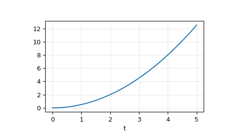
In a second example, we simulate a double integrator y'' = u, with a constant input u = 1. We’ll use the state space representation of the integrator.

>>> from scipy.signal import lti
>>> A = np.array([[0.0, 1.0], [0.0, 0.0]])
>>> B = np.array([[0.0], [1.0]])
>>> C = np.array([[1.0, 0.0]])
>>> D = 0.0
>>> system = lti(A, B, C, D)

t and u define the time and input signal for the system to be simulated.

>>> t = np.linspace(0, 5, num=50)
>>> u = np.ones_like(t)

Compute the simulation, and then plot y. As expected, the plot shows the curve y = 0.5*t**2.

>>> tout, y, x = lsim(system, u, t)
>>> plt.plot(t, y)
>>> plt.grid(alpha=0.3)
>>> plt.xlabel('t')
>>> plt.show()