scipy.stats.hypergeom
-
scipy.stats.hypergeom= <scipy.stats._discrete_distns.hypergeom_gen object>[source]¶ A hypergeometric discrete random variable.
The hypergeometric distribution models drawing objects from a bin. M is the total number of objects, n is total number of Type I objects. The random variate represents the number of Type I objects in N drawn without replacement from the total population.
As an instance of the
rv_discreteclass,hypergeomobject inherits from it a collection of generic methods (see below for the full list), and completes them with details specific for this particular distribution.Notes
The symbols used to denote the shape parameters (M, n, and N) are not universally accepted. See the Examples for a clarification of the definitions used here.
The probability mass function is defined as,
\[p(k, M, n, N) = \frac{\binom{n}{k} \binom{M - n}{N - k}} {\binom{M}{N}}\]for \(k \in [\max(0, N - M + n), \min(n, N)]\), where the binomial coefficients are defined as,
\[\binom{n}{k} \equiv \frac{n!}{k! (n - k)!}.\]The probability mass function above is defined in the “standardized” form. To shift distribution use the
locparameter. Specifically,hypergeom.pmf(k, M, n, N, loc)is identically equivalent tohypergeom.pmf(k - loc, M, n, N).Examples
>>> from scipy.stats import hypergeom
>>> import matplotlib.pyplot as plt
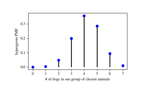
Suppose we have a collection of 20 animals, of which 7 are dogs. Then if we want to know the probability of finding a given number of dogs if we choose at random 12 of the 20 animals, we can initialize a frozen distribution and plot the probability mass function:
>>> [M, n, N] = [20, 7, 12]
>>> rv = hypergeom(M, n, N)
>>> x = np.arange(0, n+1)
>>> pmf_dogs = rv.pmf(x)
>>> fig = plt.figure()
>>> ax = fig.add_subplot(111)
>>> ax.plot(x, pmf_dogs, 'bo')
>>> ax.vlines(x, 0, pmf_dogs, lw=2)
>>> ax.set_xlabel('# of dogs in our group of chosen animals')
>>> ax.set_ylabel('hypergeom PMF')
>>> plt.show()
Instead of using a frozen distribution we can also use
hypergeommethods directly. To for example obtain the cumulative distribution function, use:>>> prb = hypergeom.cdf(x, M, n, N)
And to generate random numbers:
>>> R = hypergeom.rvs(M, n, N, size=10)
Methods
rvs(M, n, N, loc=0, size=1, random_state=None) Random variates. pmf(k, M, n, N, loc=0) Probability mass function. logpmf(k, M, n, N, loc=0) Log of the probability mass function. cdf(k, M, n, N, loc=0) Cumulative distribution function. logcdf(k, M, n, N, loc=0) Log of the cumulative distribution function. sf(k, M, n, N, loc=0) Survival function (also defined as 1 - cdf, but sf is sometimes more accurate).logsf(k, M, n, N, loc=0) Log of the survival function. ppf(q, M, n, N, loc=0) Percent point function (inverse of cdf— percentiles).isf(q, M, n, N, loc=0) Inverse survival function (inverse of sf).stats(M, n, N, loc=0, moments=’mv’) Mean(‘m’), variance(‘v’), skew(‘s’), and/or kurtosis(‘k’). entropy(M, n, N, loc=0) (Differential) entropy of the RV. expect(func, args=(M, n, N), loc=0, lb=None, ub=None, conditional=False) Expected value of a function (of one argument) with respect to the distribution. median(M, n, N, loc=0) Median of the distribution. mean(M, n, N, loc=0) Mean of the distribution. var(M, n, N, loc=0) Variance of the distribution. std(M, n, N, loc=0) Standard deviation of the distribution. interval(alpha, M, n, N, loc=0) Endpoints of the range that contains alpha percent of the distribution