scipy.signal.lsim
-
scipy.signal.lsim(system, U, T, X0=None, interp=True)[source]¶ Simulate output of a continuous-time linear system.
Parameters: - system : an instance of the LTI class or a tuple describing the system.
The following gives the number of elements in the tuple and the interpretation:
- 1: (instance of
lti) - 2: (num, den)
- 3: (zeros, poles, gain)
- 4: (A, B, C, D)
- 1: (instance of
- U : array_like
An input array describing the input at each time T (interpolation is assumed between given times). If there are multiple inputs, then each column of the rank-2 array represents an input. If U = 0 or None, a zero input is used.
- T : array_like
The time steps at which the input is defined and at which the output is desired. Must be nonnegative, increasing, and equally spaced.
- X0 : array_like, optional
The initial conditions on the state vector (zero by default).
- interp : bool, optional
Whether to use linear (True, the default) or zero-order-hold (False) interpolation for the input array.
Returns: - T : 1D ndarray
Time values for the output.
- yout : 1D ndarray
System response.
- xout : ndarray
Time evolution of the state vector.
Notes
If (num, den) is passed in for
system, coefficients for both the numerator and denominator should be specified in descending exponent order (e.g.s^2 + 3s + 5would be represented as[1, 3, 5]).Examples
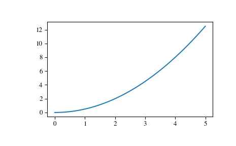
Simulate a double integrator y’’ = u, with a constant input u = 1
>>> from scipy import signal
>>> system = signal.lti([[0., 1.], [0., 0.]], [[0.], [1.]], [[1., 0.]], 0.)
>>> t = np.linspace(0, 5)
>>> u = np.ones_like(t)
>>> tout, y, x = signal.lsim(system, u, t)
>>> import matplotlib.pyplot as plt
>>> plt.plot(t, y)

