scipy.signal.sosfreqz
-
scipy.signal.sosfreqz(sos, worN=None, whole=False)[source]¶ Compute the frequency response of a digital filter in SOS format.
Given sos, an array with shape (n, 6) of second order sections of a digital filter, compute the frequency response of the system function:
       B0(z)   B1(z)         B{n-1}(z)
H(z) = ----- * ----- * ... * ---------
       A0(z)   A1(z)         A{n-1}(z)
for z = exp(omega*1j), where B{k}(z) and A{k}(z) are numerator and denominator of the transfer function of the k-th second order section.
Parameters: sos : array_like
Array of second-order filter coefficients, must have shape
(n_sections, 6). Each row corresponds to a second-order section, with the first three columns providing the numerator coefficients and the last three providing the denominator coefficients.worN : {None, int, array_like}, optional
If None (default), then compute at 512 frequencies equally spaced around the unit circle. If a single integer, then compute at that many frequencies. Using a number that is fast for FFT computations can result in faster computations (see Notes of
freqz). If an array_like, compute the response at the frequencies given (in radians/sample; must be 1D).whole : bool, optional
Normally, frequencies are computed from 0 to the Nyquist frequency, pi radians/sample (upper-half of unit-circle). If whole is True, compute frequencies from 0 to 2*pi radians/sample.
Returns: w : ndarray
The normalized frequencies at which h was computed, in radians/sample.
h : ndarray
The frequency response, as complex numbers.
Notes
New in version 0.19.0.
Examples
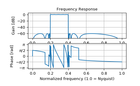
Design a 15th-order bandpass filter in SOS format.
>>> from scipy import signal
>>> sos = signal.ellip(15, 0.5, 60, (0.2, 0.4), btype='bandpass',
...                    output='sos')
Compute the frequency response at 1500 points from DC to Nyquist.
>>> w, h = signal.sosfreqz(sos, worN=1500)
Plot the response.
>>> import matplotlib.pyplot as plt
>>> plt.subplot(2, 1, 1)
>>> db = 20*np.log10(np.abs(h))
>>> plt.plot(w/np.pi, db)
>>> plt.ylim(-75, 5)
>>> plt.grid(True)
>>> plt.yticks([0, -20, -40, -60])
>>> plt.ylabel('Gain [dB]')
>>> plt.title('Frequency Response')
>>> plt.subplot(2, 1, 2)
>>> plt.plot(w/np.pi, np.angle(h))
>>> plt.grid(True)
>>> plt.yticks([-np.pi, -0.5*np.pi, 0, 0.5*np.pi, np.pi],
...            [r'$-\pi$', r'$-\pi/2$', '0', r'$\pi/2$', r'$\pi$'])
>>> plt.ylabel('Phase [rad]')
>>> plt.xlabel('Normalized frequency (1.0 = Nyquist)')
>>> plt.show()
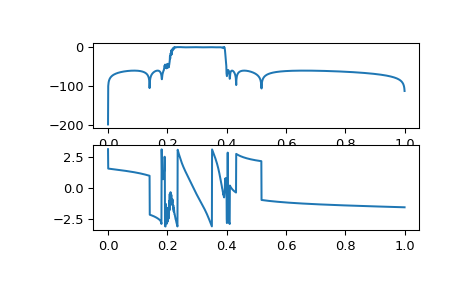
If the same filter is implemented as a single transfer function, numerical error corrupts the frequency response:
>>> b, a = signal.ellip(15, 0.5, 60, (0.2, 0.4), btype='bandpass',
...                    output='ba')
>>> w, h = signal.freqz(b, a, worN=1500)
>>> plt.subplot(2, 1, 1)
>>> db = 20*np.log10(np.abs(h))
>>> plt.plot(w/np.pi, db)
>>> plt.subplot(2, 1, 2)
>>> plt.plot(w/np.pi, np.angle(h))
>>> plt.show()