scipy.signal.freqs_zpk
-
scipy.signal.freqs_zpk(z, p, k, worN=None)[source]¶ Compute frequency response of analog filter.
Given the zeros z, poles p, and gain k of a filter, compute its frequency response:
           (jw-z[0]) * (jw-z[1]) * ... * (jw-z[-1])
H(w) = k * ----------------------------------------
           (jw-p[0]) * (jw-p[1]) * ... * (jw-p[-1])
Parameters: z : array_like
Zeroes of a linear filter
p : array_like
Poles of a linear filter
k : scalar
Gain of a linear filter
worN : {None, int, array_like}, optional
If None, then compute at 200 frequencies around the interesting parts of the response curve (determined by pole-zero locations). If a single integer, then compute at that many frequencies. Otherwise, compute the response at the angular frequencies (e.g. rad/s) given in worN.
Returns: w : ndarray
The angular frequencies at which h was computed.
h : ndarray
The frequency response.
See also
Notes
Examples
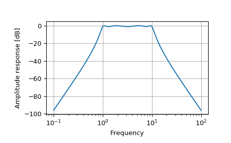
>>> from scipy.signal import freqs_zpk, iirfilter
>>> z, p, k = iirfilter(4, [1, 10], 1, 60, analog=True, ftype='cheby1',
...                     output='zpk')
>>> w, h = freqs_zpk(z, p, k, worN=np.logspace(-1, 2, 1000))
>>> import matplotlib.pyplot as plt
>>> plt.semilogx(w, 20 * np.log10(abs(h)))
>>> plt.xlabel('Frequency')
>>> plt.ylabel('Amplitude response [dB]')
>>> plt.grid()
>>> plt.show()