scipy.signal.cheb1ord
-
scipy.signal.cheb1ord(wp, ws, gpass, gstop, analog=False)[source]¶ Chebyshev type I filter order selection.
Return the order of the lowest order digital or analog Chebyshev Type I filter that loses no more than gpass dB in the passband and has at least gstop dB attenuation in the stopband.
Parameters: wp, ws : float
Passband and stopband edge frequencies. For digital filters, these are normalized from 0 to 1, where 1 is the Nyquist frequency, pi radians/sample. (wp and ws are thus in half-cycles / sample.) For example:
- Lowpass: wp = 0.2, ws = 0.3
- Highpass: wp = 0.3, ws = 0.2
- Bandpass: wp = [0.2, 0.5], ws = [0.1, 0.6]
- Bandstop: wp = [0.1, 0.6], ws = [0.2, 0.5]
For analog filters, wp and ws are angular frequencies (e.g. rad/s).
gpass : float
The maximum loss in the passband (dB).
gstop : float
The minimum attenuation in the stopband (dB).
analog : bool, optional
When True, return an analog filter, otherwise a digital filter is returned.
Returns: ord : int
The lowest order for a Chebyshev type I filter that meets specs.
wn : ndarray or float
The Chebyshev natural frequency (the “3dB frequency”) for use with
cheby1to give filter results.See also
Examples
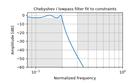
Design a digital lowpass filter such that the passband is within 3 dB up to 0.2*(fs/2), while rejecting at least -40 dB above 0.3*(fs/2). Plot its frequency response, showing the passband and stopband constraints in gray.
>>> from scipy import signal
>>> import matplotlib.pyplot as plt
>>> N, Wn = signal.cheb1ord(0.2, 0.3, 3, 40)
>>> b, a = signal.cheby1(N, 3, Wn, 'low')
>>> w, h = signal.freqz(b, a)
>>> plt.semilogx(w / np.pi, 20 * np.log10(abs(h)))
>>> plt.title('Chebyshev I lowpass filter fit to constraints')
>>> plt.xlabel('Normalized frequency')
>>> plt.ylabel('Amplitude [dB]')
>>> plt.grid(which='both', axis='both')
>>> plt.fill([.01, 0.2, 0.2, .01], [-3, -3, -99, -99], '0.9', lw=0) # stop
>>> plt.fill([0.3, 0.3,   2,   2], [ 9, -40, -40,  9], '0.9', lw=0) # pass
>>> plt.axis([0.08, 1, -60, 3])
>>> plt.show()