scipy.ndimage.uniform_filter
-
scipy.ndimage.uniform_filter(input, size=3, output=None, mode='reflect', cval=0.0, origin=0)[source]¶ Multi-dimensional uniform filter.
Parameters: input : array_like
Input array to filter.
size : int or sequence of ints, optional
The sizes of the uniform filter are given for each axis as a sequence, or as a single number, in which case the size is equal for all axes.
output : array, optional
The output parameter passes an array in which to store the filter output. Output array should have different name as compared to input array to avoid aliasing errors.
mode : str or sequence, optional
The mode parameter determines how the array borders are handled. Valid modes are {‘reflect’, ‘constant’, ‘nearest’, ‘mirror’, ‘wrap’}. cval is the value used when mode is equal to ‘constant’. A list of modes with length equal to the number of axes can be provided to specify different modes for different axes. Default is ‘reflect’
cval : scalar, optional
Value to fill past edges of input if mode is ‘constant’. Default is 0.0
origin : scalar, optional
The origin parameter controls the placement of the filter. Default 0.0.
Returns: uniform_filter : ndarray
Filtered array. Has the same shape as input.
Notes
The multi-dimensional filter is implemented as a sequence of one-dimensional uniform filters. The intermediate arrays are stored in the same data type as the output. Therefore, for output types with a limited precision, the results may be imprecise because intermediate results may be stored with insufficient precision.
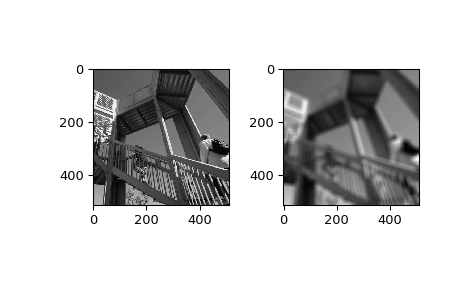
Examples
>>> from scipy import ndimage, misc
>>> import matplotlib.pyplot as plt
>>> fig = plt.figure()
>>> plt.gray()  # show the filtered result in grayscale
>>> ax1 = fig.add_subplot(121)  # left side
>>> ax2 = fig.add_subplot(122)  # right side
>>> ascent = misc.ascent()
>>> result = ndimage.uniform_filter(ascent, size=20)
>>> ax1.imshow(ascent)
>>> ax2.imshow(result)
>>> plt.show()