scipy.ndimage.gaussian_filter1d
-
scipy.ndimage.gaussian_filter1d(input, sigma, axis=-1, order=0, output=None, mode='reflect', cval=0.0, truncate=4.0)[source]¶ One-dimensional Gaussian filter.
Parameters: input : array_like
Input array to filter.
sigma : scalar
standard deviation for Gaussian kernel
axis : int, optional
The axis of input along which to calculate. Default is -1.
order : int, optional
An order of 0 corresponds to convolution with a Gaussian kernel. A positive order corresponds to convolution with that derivative of a Gaussian.
output : array, optional
The output parameter passes an array in which to store the filter output. Output array should have different name as compared to input array to avoid aliasing errors.
mode : {‘reflect’, ‘constant’, ‘nearest’, ‘mirror’, ‘wrap’}, optional
The mode parameter determines how the array borders are handled, where cval is the value when mode is equal to ‘constant’. Default is ‘reflect’
cval : scalar, optional
Value to fill past edges of input if mode is ‘constant’. Default is 0.0
truncate : float, optional
Truncate the filter at this many standard deviations. Default is 4.0.
Returns: gaussian_filter1d : ndarray
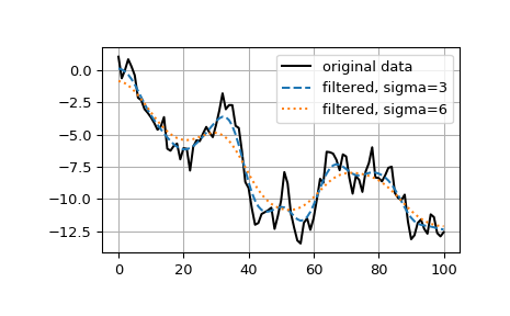
Examples
>>> from scipy.ndimage import gaussian_filter1d
>>> gaussian_filter1d([1.0, 2.0, 3.0, 4.0, 5.0], 1)
array([ 1.42704095,  2.06782203,  3.        ,  3.93217797,  4.57295905])
>>> gaussian_filter1d([1.0, 2.0, 3.0, 4.0, 5.0], 4)
array([ 2.91948343,  2.95023502,  3.        ,  3.04976498,  3.08051657])
>>> import matplotlib.pyplot as plt
>>> np.random.seed(280490)
>>> x = np.random.randn(101).cumsum()
>>> y3 = gaussian_filter1d(x, 3)
>>> y6 = gaussian_filter1d(x, 6)
>>> plt.plot(x, 'k', label='original data')
>>> plt.plot(y3, '--', label='filtered, sigma=3')
>>> plt.plot(y6, ':', label='filtered, sigma=6')
>>> plt.legend()
>>> plt.grid()
>>> plt.show()