Discrete Statistical Distributions
Discrete random variables take on only a countable number of values.
The commonly used distributions are included in SciPy and described in
this document. Each discrete distribution can take one extra integer
parameter:  The relationship between the general distribution
 and the standard distribution
  is
is
![\[ p\left(x\right)=p_{0}\left(x-L\right)\]](../../_images/math/053d0eb2c714237240033c3ee41a4d0ed2ce60c2.png)
which allows for shifting of the input. When a distribution generator
is initialized, the discrete distribution can either specify the
beginning and ending (integer) values  and
and  which must be such that
![\[ p_{0}\left(x\right)=0\quad x<a\textrm{ or }x>b\]](../../_images/math/10e3ca280d4bd2213cf961e6e67fda52d987a83a.png)
in which case, it is assumed that the pdf function is specified on the
integers  where
where  is a non-negative integer (
  ) and
) and  is a positive integer multiplier. Alternatively, the two lists
  and
and  can be provided directly in which case a dictionary is set up
internally to evaulate probabilities and generate random variates.
can be provided directly in which case a dictionary is set up
internally to evaulate probabilities and generate random variates.
Probability Mass Function (PMF)
The probability mass function of a random variable X is defined as the probability that the random variable takes on a particular value.
![\[ p\left(x_{k}\right)=P\left[X=x_{k}\right]\]](../../_images/math/553785308262819d437a05525c46eb06831444e7.png)
This is also sometimes called the probability density function, although technically
![\[ f\left(x\right)=\sum_{k}p\left(x_{k}\right)\delta\left(x-x_{k}\right)\]](../../_images/math/9c8c55dae36f2da835f91dc73b60869d90367095.png)
is the probability density function for a discrete distribution [1] .
| [1] | XXX: Unknown layout Plain Layout: Note that we will be using to represent the probability mass function and a parameter (a
XXX: probability). The usage should be obvious from context. |
Cumulative Distribution Function (CDF)
The cumulative distribution function is
![\[ F\left(x\right)=P\left[X\leq x\right]=\sum_{x_{k}\leq x}p\left(x_{k}\right)\]](../../_images/math/9f21c6030b9cfe78c591037c672da190f6386fe3.png)
and is also useful to be able to compute. Note that
![\[ F\left(x_{k}\right)-F\left(x_{k-1}\right)=p\left(x_{k}\right)\]](../../_images/math/f3a1068a264dc5572573faead93466da3cb9ff17.png)
Survival Function
The survival function is just
![\[ S\left(x\right)=1-F\left(x\right)=P\left[X>k\right]\]](../../_images/math/ddabab393c853db82fd59a95f93e9353c022049f.png)
the probability that the random variable is strictly larger than .
Percent Point Function (Inverse CDF)
The percent point function is the inverse of the cumulative distribution function and is
![\[ G\left(q\right)=F^{-1}\left(q\right)\]](../../_images/math/78b011bf6980d18b73a1875db2267bc50f6d7aec.png)
for discrete distributions, this must be modified for cases where
there is no such that  In these cases we choose
  to be the smallest value
  for which
  . If
. If  then we define
  . This definition allows random variates to be defined in the same way
as with continuous rv’s using the inverse cdf on a uniform
distribution to generate random variates.
. This definition allows random variates to be defined in the same way
as with continuous rv’s using the inverse cdf on a uniform
distribution to generate random variates.
Inverse survival function
The inverse survival function is the inverse of the survival function
![\[ Z\left(\alpha\right)=S^{-1}\left(\alpha\right)=G\left(1-\alpha\right)\]](../../_images/math/fb59d6a2f136a21aba69e23458178a67afc6533a.png)
and is thus the smallest non-negative integer for which  or the smallest non-negative integer for which
Hazard functions
If desired, the hazard function and the cumulative hazard function could be defined as
![\[ h\left(x_{k}\right)=\frac{p\left(x_{k}\right)}{1-F\left(x_{k}\right)}\]](../../_images/math/43fde823c8d0eabe34801c18ae60940e6860709e.png)
and
![\[ H\left(x\right)=\sum_{x_{k}\leq x}h\left(x_{k}\right)=\sum_{x_{k}\leq x}\frac{F\left(x_{k}\right)-F\left(x_{k-1}\right)}{1-F\left(x_{k}\right)}.\]](../../_images/math/fcf0e6c9670aaf3369a3948179e99bcf280bbfcd.png)
Moments
Non-central moments are defined using the PDF
![\[ \mu_{m}^{\prime}=E\left[X^{m}\right]=\sum_{k}x_{k}^{m}p\left(x_{k}\right).\]](../../_images/math/f38c778ac59d2c3a01f1263761f034327041a7ce.png)
Central moments are computed similarly 
![\begin{eqnarray*} \mu_{m}=E\left[\left(X-\mu\right)^{m}\right] & = & \sum_{k}\left(x_{k}-\mu\right)^{m}p\left(x_{k}\right)\\ & = & \sum_{k=0}^{m}\left(-1\right)^{m-k}\left(\begin{array}{c} m\\ k\end{array}\right)\mu^{m-k}\mu_{k}^{\prime}\end{eqnarray*}](../../_images/math/c825227ccbcd7d6eab8f2a5957491cf061b2d4bf.png)
The mean is the first moment
![\[ \mu=\mu_{1}^{\prime}=E\left[X\right]=\sum_{k}x_{k}p\left(x_{k}\right)\]](../../_images/math/a43a87d2a94b7a964282fc7471ec21b3baef2ac4.png)
the variance is the second central moment
![\[ \mu_{2}=E\left[\left(X-\mu\right)^{2}\right]=\sum_{x_{k}}x_{k}^{2}p\left(x_{k}\right)-\mu^{2}.\]](../../_images/math/c3da411d195ee947b9325858c494e7831be9e13f.png)
Skewness is defined as
![\[ \gamma_{1}=\frac{\mu_{3}}{\mu_{2}^{3/2}}\]](../../_images/math/b5ccec36e8466d5349b87fe24d39d4ce3d3b6fa6.png)
while (Fisher) kurtosis is
![\[ \gamma_{2}=\frac{\mu_{4}}{\mu_{2}^{2}}-3,\]](../../_images/math/346cb35b367ce64d9a77f072b450e58e6060b5fb.png)
so that a normal distribution has a kurtosis of zero.
Moment generating function
The moment generating funtion is defined as
![\[ M_{X}\left(t\right)=E\left[e^{Xt}\right]=\sum_{x_{k}}e^{x_{k}t}p\left(x_{k}\right)\]](../../_images/math/b33980dd5d1d250b587d22cdf7af800202783639.png)
Moments are found as the derivatives of the moment generating function
evaluated at 
Fitting data
To fit data to a distribution, maximizing the likelihood function is common. Alternatively, some distributions have well-known minimum variance unbiased estimators. These will be chosen by default, but the likelihood function will always be available for minimizing.
If  is the PDF of a random-variable where
  is a vector of parameters ( e.g.
  and
and  ), then for a collection of
  independent samples from this distribution, the joint distribution the
random vector
independent samples from this distribution, the joint distribution the
random vector  is
is
![\[ f\left(\mathbf{k};\boldsymbol{\theta}\right)=\prod_{i=1}^{N}f_{i}\left(k_{i};\boldsymbol{\theta}\right).\]](../../_images/math/e0e74c0a1083735b463f72cf41d1c251617b466a.png)
The maximum likelihood estimate of the parameters are the parameters which maximize this function with  fixed and given by the data:
Where
![\[ \overline{y\left(\mathbf{x}\right)}=\frac{1}{N}\sum_{i=1}^{N}y\left(x_{i}\right)\]](../../_images/math/60e2681c8f04d34cb42d1cee141f81436190dad8.png)
Combinations
Note that
![\[ k!=k\cdot\left(k-1\right)\cdot\left(k-2\right)\cdot\cdots\cdot1=\Gamma\left(k+1\right)\]](../../_images/math/6e25469f7db542e990b98e4ec590ef587b1c788c.png)
and has special cases of
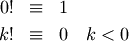
and
![\[ \left(\begin{array}{c} n\\ k\end{array}\right)=\frac{n!}{\left(n-k\right)!k!}.\]](../../_images/math/c3dbacf2fd369dcccdbbfb2ff81a6c8519604b2c.png)
If  or
or  or
or  we define
Bernoulli
A Bernoulli random variable of parameter takes one of only two values  or
or  . The probability of success ( ) is , and the probability of failure ( ) is
  It can be thought of as a binomial random variable with
  . The PMF is
  for
for  and
and
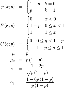
![\[ M\left(t\right)=1-p\left(1-e^{t}\right)\]](../../_images/math/64e210e61ef7b22e2160b86106c09956d6d744c2.png)
![\[ \mu_{m}^{\prime}=p\]](../../_images/math/eaa152e30abc7e5b56ba9f22960df2af7103c4dc.png)
![\[ h\left[X\right]=p\log p+\left(1-p\right)\log\left(1-p\right)\]](../../_images/math/c537e87ead7548bec393a262b458c5a26896a5bf.png)
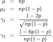
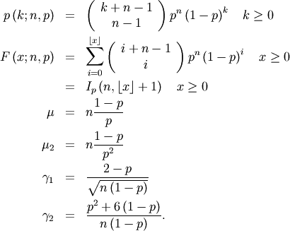
Binomial
A binomial random variable with parameters  can be described as the sum of
  independent Bernoulli random variables of parameter
![\[ Y=\sum_{i=1}^{n}X_{i}.\]](../../_images/math/2758fbc02a46a37f14c2b42d119850f1d9c3be4f.png)
Therefore, this random variable counts the number of successes in independent trials of a random experiment where the probability of
success is 
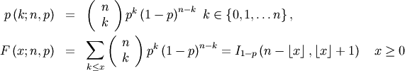
where the incomplete beta integral is
![\[ I_{x}\left(a,b\right)=\frac{\Gamma\left(a+b\right)}{\Gamma\left(a\right)\Gamma\left(b\right)}\int_{0}^{x}t^{a-1}\left(1-t\right)^{b-1}dt.\]](../../_images/math/a13bf66ecf3c96a1b23954bee92be123b59ac0c2.png)
Now
![\[ M\left(t\right)=\left[1-p\left(1-e^{t}\right)\right]^{n}\]](../../_images/math/2b422facd428573b4f89130c0647b0b7914783ca.png)
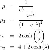
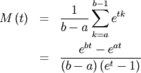
![\begin{eqnarray*} p\left(k;N,\lambda\right) & = & \frac{1-e^{-\lambda}}{1-e^{-\lambda N}}\exp\left(-\lambda k\right)\quad k\in\left\{ 0,1,\ldots,N-1\right\} \\ F\left(x;N,\lambda\right) & = & \left\{ \begin{array}{cc} 0 & x<0\\ \frac{1-\exp\left[-\lambda\left(\left\lfloor x\right\rfloor +1\right)\right]}{1-\exp\left(-\lambda N\right)} & 0\leq x\leq N-1\\ 1 & x\geq N-1\end{array}\right.\\ G\left(q,\lambda\right) & = & \left\lceil -\frac{1}{\lambda}\log\left[1-q\left(1-e^{-\lambda N}\right)\right]-1\right\rceil \end{eqnarray*}](../../_images/math/98be7ed3547ec5929f5cdcf735ed2e40210adba6.png)

![\begin{eqnarray*} \mu & = & \frac{z}{1-z}-\frac{Nz^{N}}{1-z^{N}}\\ \mu_{2} & = & \frac{z}{\left(1-z\right)^{2}}-\frac{N^{2}z^{N}}{\left(1-z^{N}\right)^{2}}\\ \gamma_{1} & = & \frac{z\left(1+z\right)\left(\frac{1-z^{N}}{1-z}\right)^{3}-N^{3}z^{N}\left(1+z^{N}\right)}{\left[z\left(\frac{1-z^{N}}{1-z}\right)^{2}-N^{2}z^{N}\right]^{3/2}}\\ \gamma_{2} & = & \frac{z\left(1+4z+z^{2}\right)\left(\frac{1-z^{N}}{1-z}\right)^{4}-N^{4}z^{N}\left(1+4z^{N}+z^{2N}\right)}{\left[z\left(\frac{1-z^{N}}{1-z}\right)^{2}-N^{2}z^{N}\right]^{2}}\end{eqnarray*}](../../_images/math/6c5bf47cd8055dfaa52eb38c1991caeabe0fb830.png)
![\[ M\left(t\right)=\frac{1-e^{N\left(t-\lambda\right)}}{1-e^{t-\lambda}}\frac{1-e^{-\lambda}}{1-e^{-\lambda N}}\]](../../_images/math/47e0b97f00c7a2d348275882a7f1244c43504301.png)
Planck (discrete exponential)
Named Planck because of its relationship to the black-body problem he solved.
![\begin{eqnarray*} p\left(k;\lambda\right) & = & \left(1-e^{-\lambda}\right)e^{-\lambda k}\quad k\lambda\geq0\\ F\left(x;\lambda\right) & = & 1-e^{-\lambda\left(\left\lfloor x\right\rfloor +1\right)}\quad x\lambda\geq0\\ G\left(q;\lambda\right) & = & \left\lceil -\frac{1}{\lambda}\log\left[1-q\right]-1\right\rceil .\end{eqnarray*}](../../_images/math/e121ee51147b8a8b0d7ade8f623336d9176cd311.png)
![\[ M\left(t\right)=\frac{1-e^{-\lambda}}{1-e^{t-\lambda}}\]](../../_images/math/1881465064a36e5ed18e50fc8dfb59dc6028b42b.png)
![\[ h\left[X\right]=\frac{\lambda e^{-\lambda}}{1-e^{-\lambda}}-\log\left(1-e^{-\lambda}\right)\]](../../_images/math/42e79ca06ba63fbe9215167ce85eb56209c12da0.png)
Poisson
The Poisson random variable counts the number of successes in independent Bernoulli trials in the limit as  and
and  where the probability of success in each trial is and
  is a constant. It can be used to approximate the Binomial random
variable or in it’s own right to count the number of events that occur
in the interval
is a constant. It can be used to approximate the Binomial random
variable or in it’s own right to count the number of events that occur
in the interval ![\left[0,t\right]](../../_images/math/f01fd7606b284644a37301160b37bcf46d45cfa3.png) for a process satisfying certain “sparsity “constraints. The functions are
for a process satisfying certain “sparsity “constraints. The functions are
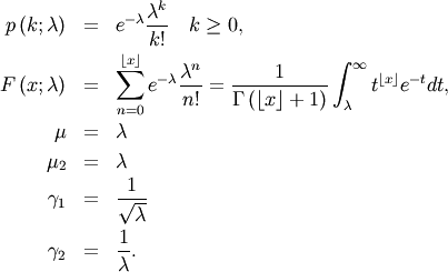
![\[ M\left(t\right)=\exp\left[\lambda\left(e^{t}-1\right)\right].\]](../../_images/math/f947b30ec15a3f50819ed543f039c1f5719ebc31.png)
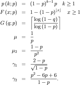
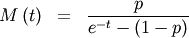
Geometric
The geometric random variable with parameter  can be defined as the number of trials required to obtain a success
where the probability of success on each trial is . Thus,
can be defined as the number of trials required to obtain a success
where the probability of success on each trial is . Thus,
Negative Binomial
The negative binomial random variable with parameters and can be defined as the number of extra independent trials (beyond ) required to accumulate a total of successes where the probability of a success on each trial is Equivalently, this random variable is the number of failures
encoutered while accumulating successes during independent trials of an experiment that succeeds
with probability Thus,
Recall that  is the incomplete beta integral.
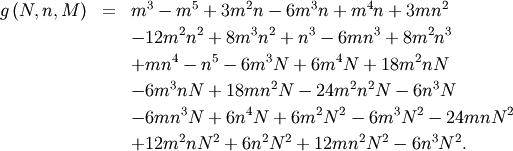
Hypergeometric
The hypergeometric random variable with parameters  counts the number of “good “objects in a sample of size chosen without replacement from a population of
  objects where is the number of “good “objects in the total population.
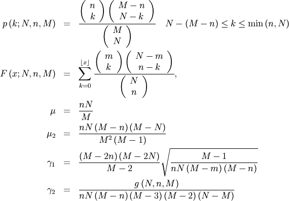
where (defining  )
)
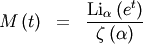
Zipf (Zeta)
A random variable has the zeta distribution (also called the zipf
distribution) with parameter  if it’s probability mass function is given by
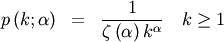
where
![\[ \zeta\left(\alpha\right)=\sum_{n=1}^{\infty}\frac{1}{n^{\alpha}}\]](../../_images/math/85be0c97af0cbcb56fde029bd9604821e6e4de18.png)
is the Riemann zeta function. Other functions of this distribution are
![\begin{eqnarray*} F\left(x;\alpha\right) & = & \frac{1}{\zeta\left(\alpha\right)}\sum_{k=1}^{\left\lfloor x\right\rfloor }\frac{1}{k^{\alpha}}\\ \mu & = & \frac{\zeta_{1}}{\zeta_{0}}\quad\alpha>2\\ \mu_{2} & = & \frac{\zeta_{2}\zeta_{0}-\zeta_{1}^{2}}{\zeta_{0}^{2}}\quad\alpha>3\\ \gamma_{1} & = & \frac{\zeta_{3}\zeta_{0}^{2}-3\zeta_{0}\zeta_{1}\zeta_{2}+2\zeta_{1}^{3}}{\left[\zeta_{2}\zeta_{0}-\zeta_{1}^{2}\right]^{3/2}}\quad\alpha>4\\ \gamma_{2} & = & \frac{\zeta_{4}\zeta_{0}^{3}-4\zeta_{3}\zeta_{1}\zeta_{0}^{2}+12\zeta_{2}\zeta_{1}^{2}\zeta_{0}-6\zeta_{1}^{4}-3\zeta_{2}^{2}\zeta_{0}^{2}}{\left(\zeta_{2}\zeta_{0}-\zeta_{1}^{2}\right)^{2}}.\end{eqnarray*}](../../_images/math/0ceb5a27d26e2be8e9611890d85ab90f20a99b00.png)
where  and
and  is the
  polylogarithm function of
  defined as
![\[ \textrm{Li}_{n}\left(z\right)\equiv\sum_{k=1}^{\infty}\frac{z^{k}}{k^{n}}\]](../../_images/math/228346a20c361fd78cff7e9767617b9a27db8aae.png)
![\[ \mu_{n}^{\prime}=\left.M^{\left(n\right)}\left(t\right)\right|_{t=0}=\left.\frac{\textrm{Li}_{\alpha-n}\left(e^{t}\right)}{\zeta\left(a\right)}\right|_{t=0}=\frac{\zeta\left(\alpha-n\right)}{\zeta\left(\alpha\right)}\]](../../_images/math/c1bae94050ff138a04705e2e3b67b8dc60cacf1a.png)
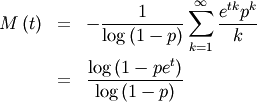
Logarithmic (Log-Series, Series)
The logarimthic distribution with parameter has a probability mass function with terms proportional to the Taylor
series expansion of 
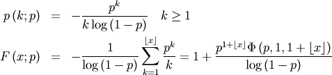
where
![\[ \Phi\left(z,s,a\right)=\sum_{k=0}^{\infty}\frac{z^{k}}{\left(a+k\right)^{s}}\]](../../_images/math/b706279a5e18e00eef82f824e8fda8079e7343e1.png)
is the Lerch Transcendent. Also define 
![\begin{eqnarray*} \mu & = & -\frac{p}{\left(1-p\right)r}\\ \mu_{2} & = & -\frac{p\left[p+r\right]}{\left(1-p\right)^{2}r^{2}}\\ \gamma_{1} & = & -\frac{2p^{2}+3pr+\left(1+p\right)r^{2}}{r\left(p+r\right)\sqrt{-p\left(p+r\right)}}r\\ \gamma_{2} & = & -\frac{6p^{3}+12p^{2}r+p\left(4p+7\right)r^{2}+\left(p^{2}+4p+1\right)r^{3}}{p\left(p+r\right)^{2}}.\end{eqnarray*}](../../_images/math/5a090fa6f38b36c8b30f3198cefc882c2e50d7d4.png)
Thus,
![\[ \mu_{n}^{\prime}=\left.M^{\left(n\right)}\left(t\right)\right|_{t=0}=\left.\frac{\textrm{Li}_{1-n}\left(pe^{t}\right)}{\log\left(1-p\right)}\right|_{t=0}=-\frac{\textrm{Li}_{1-n}\left(p\right)}{\log\left(1-p\right)}.\]](../../_images/math/39751e8194dd699b4f32df9b8f36749eef96e43b.png)
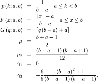
Discrete Uniform (randint)
The discrete uniform distribution with parameters  constructs a random variable that has an equal probability of being
any one of the integers in the half-open range
constructs a random variable that has an equal probability of being
any one of the integers in the half-open range  If is not given it is assumed to be zero and the only parameter is
  Therefore,
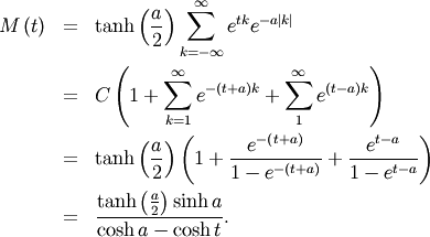
Discrete Laplacian
Defined over all integers for 
![\begin{eqnarray*} p\left(k\right) & = & \tanh\left(\frac{a}{2}\right)e^{-a\left|k\right|},\\ F\left(x\right) & = & \left\{ \begin{array}{cc} \frac{e^{a\left(\left\lfloor x\right\rfloor +1\right)}}{e^{a}+1} & \left\lfloor x\right\rfloor <0,\\ 1-\frac{e^{-a\left\lfloor x\right\rfloor }}{e^{a}+1} & \left\lfloor x\right\rfloor \geq0.\end{array}\right.\\ G\left(q\right) & = & \left\{ \begin{array}{cc} \left\lceil \frac{1}{a}\log\left[q\left(e^{a}+1\right)\right]-1\right\rceil & q<\frac{1}{1+e^{-a}},\\ \left\lceil -\frac{1}{a}\log\left[\left(1-q\right)\left(1+e^{a}\right)\right]\right\rceil & q\geq\frac{1}{1+e^{-a}}.\end{array}\right.\end{eqnarray*}](../../_images/math/5a010dd265d8c70e6d80ff9fa85f0438217b0eba.png)
Thus,
![\[ \mu_{n}^{\prime}=M^{\left(n\right)}\left(0\right)=\left[1+\left(-1\right)^{n}\right]\textrm{Li}_{-n}\left(e^{-a}\right)\]](../../_images/math/93247ecaacd168f9d5e2274fb95d6dc67daf26d3.png)
where  is the polylogarithm function of order
  evaluated at
![\[ h\left[X\right]=-\log\left(\tanh\left(\frac{a}{2}\right)\right)+\frac{a}{\sinh a}\]](../../_images/math/1b550b4afd022c5982e56bda26a5c4d194669ee0.png)
 and
and  and
and ![\[ p\left(k;\mu,\lambda\right)=\frac{1}{Z\left(\lambda\right)}\exp\left[-\lambda\left(k-\mu\right)^{2}\right]\]](../../_images/math/23f127acffd95fb6b8ecb8263c715b49fa9c442f.png)
![\[ Z\left(\lambda\right)=\sum_{k=-\infty}^{\infty}\exp\left[-\lambda k^{2}\right]\]](../../_images/math/f77b4c674d31ed96554435c8e9165eaf32a36467.png)
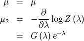
 and
and  with a minimum less than 2 near
![\[ G\left(\lambda\right)=\frac{1}{Z\left(\lambda\right)}\sum_{k=-\infty}^{\infty}k^{2}\exp\left[-\lambda\left(k+1\right)\left(k-1\right)\right]\]](../../_images/math/47d8408507e846532029b5005f276728483490dd.png)

Table Of Contents
- Discrete Statistical Distributions