scipy.signal.butter
-
scipy.signal.butter(N, Wn, btype='low', analog=False, output='ba')[source]¶ Butterworth digital and analog filter design.
Design an Nth-order digital or analog Butterworth filter and return the filter coefficients.
Parameters: N : int
The order of the filter.
Wn : array_like
A scalar or length-2 sequence giving the critical frequencies. For a Butterworth filter, this is the point at which the gain drops to 1/sqrt(2) that of the passband (the “-3 dB point”). For digital filters, Wn is normalized from 0 to 1, where 1 is the Nyquist frequency, pi radians/sample. (Wn is thus in half-cycles / sample.) For analog filters, Wn is an angular frequency (e.g. rad/s).
btype : {‘lowpass’, ‘highpass’, ‘bandpass’, ‘bandstop’}, optional
The type of filter. Default is ‘lowpass’.
analog : bool, optional
When True, return an analog filter, otherwise a digital filter is returned.
output : {‘ba’, ‘zpk’, ‘sos’}, optional
Type of output: numerator/denominator (‘ba’), pole-zero (‘zpk’), or second-order sections (‘sos’). Default is ‘ba’.
Returns: b, a : ndarray, ndarray
Numerator (b) and denominator (a) polynomials of the IIR filter. Only returned if
output='ba'.z, p, k : ndarray, ndarray, float
Zeros, poles, and system gain of the IIR filter transfer function. Only returned if
output='zpk'.sos : ndarray
Second-order sections representation of the IIR filter. Only returned if
output=='sos'.Notes
The Butterworth filter has maximally flat frequency response in the passband.
The
'sos'output parameter was added in 0.16.0.Examples
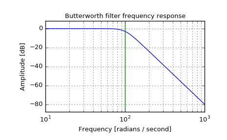
Plot the filter’s frequency response, showing the critical points:
>>> from scipy import signal
>>> import matplotlib.pyplot as plt
>>> b, a = signal.butter(4, 100, 'low', analog=True)
>>> w, h = signal.freqs(b, a)
>>> plt.semilogx(w, 20 * np.log10(abs(h)))
>>> plt.title('Butterworth filter frequency response')
>>> plt.xlabel('Frequency [radians / second]')
>>> plt.ylabel('Amplitude [dB]')
>>> plt.margins(0, 0.1)
>>> plt.grid(which='both', axis='both')
>>> plt.axvline(100, color='green') # cutoff frequency
>>> plt.show()