scipy.interpolate.make_interp_spline

scipy.interpolate.make_interp_spline(x, y, k=3, t=None, bc_type=None, axis=0, check_finite=True)

Compute the (coefficients of) interpolating B-spline.

Parameters:

x : array_like, shape (n,)

Abscissas.

y : array_like, shape (n, ...)

Ordinates.

k : int, optional

B-spline degree. Default is cubic, k=3.

t : array_like, shape (nt + k + 1,), optional.

Knots. The number of knots needs to agree with the number of datapoints and the number of derivatives at the edges. Specifically, nt - n must equal len(deriv_l) + len(deriv_r).

bc_type : 2-tuple or None

Boundary conditions. Default is None, which means choosing the boundary conditions automatically. Otherwise, it must be a length-two tuple where the first element sets the boundary conditions at x[0] and the second element sets the boundary conditions at x[-1]. Each of these must be an iterable of pairs (order, value) which gives the values of derivatives of specified orders at the given edge of the interpolation interval.

axis : int, optional

Interpolation axis. Default is 0.

check_finite : bool, optional

Whether to check that the input arrays contain only finite numbers. Disabling may give a performance gain, but may result in problems (crashes, non-termination) if the inputs do contain infinities or NaNs. Default is True.

Returns:

b : a BSpline object of the degree k and with knots t.

See also

BSpline

base class representing the B-spline objects

CubicSpline

a cubic spline in the polynomial basis

make_lsq_spline

a similar factory function for spline fitting

UnivariateSpline

a wrapper over FITPACK spline fitting routines

splrep

a wrapper over FITPACK spline fitting routines

Examples

Use cubic interpolation on Chebyshev nodes:

>>> def cheb_nodes(N):
...     jj = 2.*np.arange(N) + 1
...     x = np.cos(np.pi * jj / 2 / N)[::-1]
...     return x

>>> x = cheb_nodes(20)
>>> y = np.sqrt(1 - x**2)

>>> from scipy.interpolate import BSpline, make_interp_spline
>>> b = make_interp_spline(x, y)
>>> np.allclose(b(x), y)
True

Note that the default is a cubic spline with a not-a-knot boundary condition

>>> b.k
3

Here we use a ‘natural’ spline, with zero 2nd derivatives at edges:

>>> l, r = [(2, 0)], [(2, 0)]
>>> b_n = make_interp_spline(x, y, bc_type=(l, r))
>>> np.allclose(b_n(x), y)
True
>>> x0, x1 = x[0], x[-1]
>>> np.allclose([b_n(x0, 2), b_n(x1, 2)], [0, 0])
True

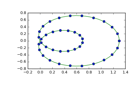
Interpolation of parametric curves is also supported. As an example, we compute a discretization of a snail curve in polar coordinates

>>> phi = np.linspace(0, 2.*np.pi, 40)
>>> r = 0.3 + np.cos(phi)
>>> x, y = r*np.cos(phi), r*np.sin(phi)  # convert to Cartesian coordinates

Build an interpolating curve, parameterizing it by the angle

>>> from scipy.interpolate import make_interp_spline
>>> spl = make_interp_spline(phi, np.c_[x, y])

Evaluate the interpolant on a finer grid (note that we transpose the result to unpack it into a pair of x- and y-arrays)

>>> phi_new = np.linspace(0, 2.*np.pi, 100)
>>> x_new, y_new = spl(phi_new).T

Plot the result

>>> import matplotlib.pyplot as plt
>>> plt.plot(x, y, 'o')
>>> plt.plot(x_new, y_new, '-')
>>> plt.show()

(Source code)