scipy.signal.convolve

scipy.signal.convolve(in1, in2, mode='full', method='auto')

Convolve two N-dimensional arrays.

Convolve in1 and in2, with the output size determined by the mode argument.

Parameters:

in1 : array_like

First input.

in2 : array_like

Second input. Should have the same number of dimensions as in1.

mode : str {‘full’, ‘valid’, ‘same’}, optional

A string indicating the size of the output:

full

The output is the full discrete linear convolution of the inputs. (Default)

valid

The output consists only of those elements that do not rely on the zero-padding. In ‘valid’ mode, either in1 or in2 must be at least as large as the other in every dimension.

same

The output is the same size as in1, centered with respect to the ‘full’ output.

method : str {‘auto’, ‘direct’, ‘fft’}, optional

A string indicating which method to use to calculate the convolution.

direct

The convolution is determined directly from sums, the definition of convolution.

fft

The Fourier Transform is used to perform the convolution by calling fftconvolve.

auto

Automatically chooses direct or Fourier method based on an estimate of which is faster (default). See Notes for more detail.

New in version 0.19.0.

Returns:

convolve : array

An N-dimensional array containing a subset of the discrete linear convolution of in1 with in2.

See also

numpy.polymul

performs polynomial multiplication (same operation, but also accepts poly1d objects)

choose_conv_method

chooses the fastest appropriate convolution method

fftconvolve

Notes

By default, convolve and correlate use method='auto', which calls choose_conv_method to choose the fastest method using pre-computed values (choose_conv_method can also measure real-world timing with a keyword argument). Because fftconvolve relies on floating point numbers, there are certain constraints that may force method=direct (more detail in choose_conv_method docstring).

Examples

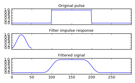
Smooth a square pulse using a Hann window:

>>> from scipy import signal
>>> sig = np.repeat([0., 1., 0.], 100)
>>> win = signal.hann(50)
>>> filtered = signal.convolve(sig, win, mode='same') / sum(win)

>>> import matplotlib.pyplot as plt
>>> fig, (ax_orig, ax_win, ax_filt) = plt.subplots(3, 1, sharex=True)
>>> ax_orig.plot(sig)
>>> ax_orig.set_title('Original pulse')
>>> ax_orig.margins(0, 0.1)
>>> ax_win.plot(win)
>>> ax_win.set_title('Filter impulse response')
>>> ax_win.margins(0, 0.1)
>>> ax_filt.plot(filtered)
>>> ax_filt.set_title('Filtered signal')
>>> ax_filt.margins(0, 0.1)
>>> fig.tight_layout()
>>> fig.show()

(Source code)