scipy.interpolate.LSQSphereBivariateSpline

class scipy.interpolate.LSQSphereBivariateSpline(theta, phi, r, tt, tp, w=None, eps=1e-16)

Weighted least-squares bivariate spline approximation in spherical coordinates.

New in version 0.11.0.

Parameters:

theta, phi, r : array_like

1-D sequences of data points (order is not important). Coordinates must be given in radians. Theta must lie within the interval (0, pi), and phi must lie within the interval (0, 2pi).

tt, tp : array_like

Strictly ordered 1-D sequences of knots coordinates. Coordinates must satisfy 0 < tt[i] < pi, 0 < tp[i] < 2*pi.

w : array_like, optional

Positive 1-D sequence of weights, of the same length as theta, phi and r.

eps : float, optional

A threshold for determining the effective rank of an over-determined linear system of equations. eps should have a value between 0 and 1, the default is 1e-16.

Notes

For more information, see the FITPACK site about this function.

Examples

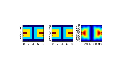
Suppose we have global data on a coarse grid (the input data does not have to be on a grid):

>>> theta = np.linspace(0., np.pi, 7)
>>> phi = np.linspace(0., 2*np.pi, 9)
>>> data = np.empty((theta.shape[0], phi.shape[0]))
>>> data[:,0], data[0,:], data[-1,:] = 0., 0., 0.
>>> data[1:-1,1], data[1:-1,-1] = 1., 1.
>>> data[1,1:-1], data[-2,1:-1] = 1., 1.
>>> data[2:-2,2], data[2:-2,-2] = 2., 2.
>>> data[2,2:-2], data[-3,2:-2] = 2., 2.
>>> data[3,3:-2] = 3.
>>> data = np.roll(data, 4, 1)

We need to set up the interpolator object. Here, we must also specify the coordinates of the knots to use.

>>> lats, lons = np.meshgrid(theta, phi)
>>> knotst, knotsp = theta.copy(), phi.copy()
>>> knotst[0] += .0001
>>> knotst[-1] -= .0001
>>> knotsp[0] += .0001
>>> knotsp[-1] -= .0001
>>> from scipy.interpolate import LSQSphereBivariateSpline
>>> lut = LSQSphereBivariateSpline(lats.ravel(), lons.ravel(),
...                                data.T.ravel(), knotst, knotsp)

As a first test, we’ll see what the algorithm returns when run on the input coordinates

>>> data_orig = lut(theta, phi)

Finally we interpolate the data to a finer grid

>>> fine_lats = np.linspace(0., np.pi, 70)
>>> fine_lons = np.linspace(0., 2*np.pi, 90)

>>> data_lsq = lut(fine_lats, fine_lons)

>>> import matplotlib.pyplot as plt
>>> fig = plt.figure()
>>> ax1 = fig.add_subplot(131)
>>> ax1.imshow(data, interpolation='nearest')
>>> ax2 = fig.add_subplot(132)
>>> ax2.imshow(data_orig, interpolation='nearest')
>>> ax3 = fig.add_subplot(133)
>>> ax3.imshow(data_lsq, interpolation='nearest')
>>> plt.show()

(Source code)

Methods

__call__(theta, phi[, dtheta, dphi, grid])	Evaluate the spline or its derivatives at given positions.
ev(theta, phi[, dtheta, dphi])	Evaluate the spline at points
get_coeffs()	Return spline coefficients.
get_knots()	Return a tuple (tx,ty) where tx,ty contain knots positions of the spline with respect to x-, y-variable, respectively.
get_residual()	Return weighted sum of squared residuals of the spline