scipy.interpolate.interp2d

class scipy.interpolate.interp2d(x, y, z, kind='linear', copy=True, bounds_error=False, fill_value=nan)

Interpolate over a 2-D grid.

x, y and z are arrays of values used to approximate some function f: z = f(x, y). This class returns a function whose call method uses spline interpolation to find the value of new points.

If x and y represent a regular grid, consider using RectBivariateSpline.

Parameters:

x, y : array_like

Arrays defining the data point coordinates.

If the points lie on a regular grid, x can specify the column coordinates and y the row coordinates, for example:

>>> x = [0,1,2];  y = [0,3]; z = [[1,2,3], [4,5,6]]

Otherwise, x and y must specify the full coordinates for each point, for example:

>>> x = [0,1,2,0,1,2];  y = [0,0,0,3,3,3]; z = [1,2,3,4,5,6]

If x and y are multi-dimensional, they are flattened before use.

z : array_like

The values of the function to interpolate at the data points. If z is a multi-dimensional array, it is flattened before use. The length of a flattened z array is either len(x)*len(y) if x and y specify the column and row coordinates or len(z) == len(x) == len(y) if x and y specify coordinates for each point.

kind : {‘linear’, ‘cubic’, ‘quintic’}, optional

The kind of spline interpolation to use. Default is ‘linear’.

copy : bool, optional

If True, the class makes internal copies of x, y and z. If False, references may be used. The default is to copy.

bounds_error : bool, optional

If True, when interpolated values are requested outside of the domain of the input data (x,y), a ValueError is raised. If False, then fill_value is used.

fill_value : number, optional

If provided, the value to use for points outside of the interpolation domain. If omitted (None), values outside the domain are extrapolated.

See also

RectBivariateSpline

Much faster 2D interpolation if your input data is on a grid

bisplrep, bisplev

BivariateSpline

a more recent wrapper of the FITPACK routines

interp1d

one dimension version of this function

Notes

The minimum number of data points required along the interpolation axis is (k+1)**2, with k=1 for linear, k=3 for cubic and k=5 for quintic interpolation.

The interpolator is constructed by bisplrep, with a smoothing factor of 0. If more control over smoothing is needed, bisplrep should be used directly.

Examples

Construct a 2-D grid and interpolate on it:

>>> from scipy import interpolate
>>> x = np.arange(-5.01, 5.01, 0.25)
>>> y = np.arange(-5.01, 5.01, 0.25)
>>> xx, yy = np.meshgrid(x, y)
>>> z = np.sin(xx**2+yy**2)
>>> f = interpolate.interp2d(x, y, z, kind='cubic')

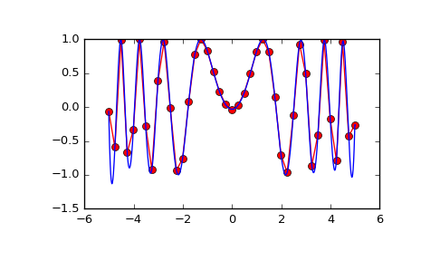
Now use the obtained interpolation function and plot the result:

>>> import matplotlib.pyplot as plt
>>> xnew = np.arange(-5.01, 5.01, 1e-2)
>>> ynew = np.arange(-5.01, 5.01, 1e-2)
>>> znew = f(xnew, ynew)
>>> plt.plot(x, z[0, :], 'ro-', xnew, znew[0, :], 'b-')
>>> plt.show()

(Source code)

Methods

__call__(x, y[, dx, dy, assume_sorted])

Interpolate the function.