scipy.signal.convolve

scipy.signal.convolve(in1, in2, mode='full')

Convolve two N-dimensional arrays.

Convolve in1 and in2, with the output size determined by the mode argument.

Parameters:

in1 : array_like

First input.

in2 : array_like

Second input. Should have the same number of dimensions as in1; if sizes of in1 and in2 are not equal then in1 has to be the larger array.

mode : str {‘full’, ‘valid’, ‘same’}, optional

A string indicating the size of the output:

full

The output is the full discrete linear convolution of the inputs. (Default)

valid

The output consists only of those elements that do not rely on the zero-padding.

same

The output is the same size as in1, centered with respect to the ‘full’ output.

Returns:

convolve : array

An N-dimensional array containing a subset of the discrete linear convolution of in1 with in2.

See also

numpy.polymul

performs polynomial multiplication (same operation, but also accepts poly1d objects)

Examples

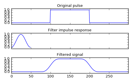
Smooth a square pulse using a Hann window:

>>> from scipy import signal
>>> sig = np.repeat([0., 1., 0.], 100)
>>> win = signal.hann(50)
>>> filtered = signal.convolve(sig, win, mode='same') / sum(win)

>>> import matplotlib.pyplot as plt
>>> fig, (ax_orig, ax_win, ax_filt) = plt.subplots(3, 1, sharex=True)
>>> ax_orig.plot(sig)
>>> ax_orig.set_title('Original pulse')
>>> ax_orig.margins(0, 0.1)
>>> ax_win.plot(win)
>>> ax_win.set_title('Filter impulse response')
>>> ax_win.margins(0, 0.1)
>>> ax_filt.plot(filtered)
>>> ax_filt.set_title('Filtered signal')
>>> ax_filt.margins(0, 0.1)
>>> fig.tight_layout()
>>> fig.show()

(Source code)