scipy.signal.exponential
- scipy.signal.exponential(M, center=None, tau=1.0, sym=True)[source]
Return an exponential (or Poisson) window.
Parameters: M : int
Number of points in the output window. If zero or less, an empty array is returned.
center : float, optional
Parameter defining the center location of the window function. The default value if not given is center = (M-1) / 2. This parameter must take its default value for symmetric windows.
tau : float, optional
Parameter defining the decay. For center = 0 use tau = -(M-1) / ln(x) if x is the fraction of the window remaining at the end.
sym : bool, optional
When True (default), generates a symmetric window, for use in filter design. When False, generates a periodic window, for use in spectral analysis.
Returns: w : ndarray
The window, with the maximum value normalized to 1 (though the value 1 does not appear if M is even and sym is True).
Notes
The Exponential window is defined as
\[w(n) = e^{-|n-center| / \tau}\]References
S. Gade and H. Herlufsen, “Windows to FFT analysis (Part I)”, Technical Review 3, Bruel & Kjaer, 1987.
Examples
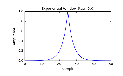
Plot the symmetric window and its frequency response:
>>> from scipy import signal
>>> from scipy.fftpack import fft, fftshift
>>> import matplotlib.pyplot as plt
>>> M = 51
>>> tau = 3.0
>>> window = signal.exponential(M, tau=tau)
>>> plt.plot(window)
>>> plt.title("Exponential Window (tau=3.0)")
>>> plt.ylabel("Amplitude")
>>> plt.xlabel("Sample")
>>> plt.figure()
>>> A = fft(window, 2048) / (len(window)/2.0)
>>> freq = np.linspace(-0.5, 0.5, len(A))
>>> response = 20 * np.log10(np.abs(fftshift(A / abs(A).max())))
>>> plt.plot(freq, response)
>>> plt.axis([-0.5, 0.5, -35, 0])
>>> plt.title("Frequency response of the Exponential window (tau=3.0)")
>>> plt.ylabel("Normalized magnitude [dB]")
>>> plt.xlabel("Normalized frequency [cycles per sample]")
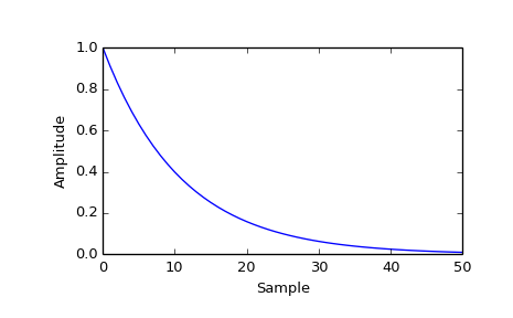
This function can also generate non-symmetric windows:
>>> tau2 = -(M-1) / np.log(0.01)
>>> window2 = signal.exponential(M, 0, tau2, False)
>>> plt.figure()
>>> plt.plot(window2)
>>> plt.ylabel("Amplitude")
>>> plt.xlabel("Sample")