scipy.signal.periodogram

scipy.signal.periodogram(x, fs=1.0, window=None, nfft=None, detrend='constant', return_onesided=True, scaling='density', axis=-1)

Estimate power spectral density using a periodogram.

Parameters:

x : array_like

Time series of measurement values

fs : float, optional

Sampling frequency of the x time series in units of Hz. Defaults to 1.0.

window : str or tuple or array_like, optional

Desired window to use. See get_window for a list of windows and required parameters. If window is an array it will be used directly as the window. Defaults to None; equivalent to ‘boxcar’.

nfft : int, optional

Length of the FFT used. If None the length of x will be used.

detrend : str or function or False, optional

Specifies how to detrend x prior to computing the spectrum. If detrend is a string, it is passed as the type argument to detrend. If it is a function, it should return a detrended array. If detrend is False, no detrending is done. Defaults to ‘constant’.

return_onesided : bool, optional

If True, return a one-sided spectrum for real data. If False return a two-sided spectrum. Note that for complex data, a two-sided spectrum is always returned.

scaling : { ‘density’, ‘spectrum’ }, optional

Selects between computing the power spectral density (‘density’) where Pxx has units of V**2/Hz if x is measured in V and computing the power spectrum (‘spectrum’) where Pxx has units of V**2 if x is measured in V. Defaults to ‘density’

axis : int, optional

Axis along which the periodogram is computed; the default is over the last axis (i.e. axis=-1).

Returns:

f : ndarray

Array of sample frequencies.

Pxx : ndarray

Power spectral density or power spectrum of x.

See also

welch

Estimate power spectral density using Welch’s method

lombscargle

Lomb-Scargle periodogram for unevenly sampled data

Notes

New in version 0.12.0.

Examples

>>> from scipy import signal
>>> import matplotlib.pyplot as plt

Generate a test signal, a 2 Vrms sine wave at 1234 Hz, corrupted by 0.001 V**2/Hz of white noise sampled at 10 kHz.

>>> fs = 10e3
>>> N = 1e5
>>> amp = 2*np.sqrt(2)
>>> freq = 1234.0
>>> noise_power = 0.001 * fs / 2
>>> time = np.arange(N) / fs
>>> x = amp*np.sin(2*np.pi*freq*time)
>>> x += np.random.normal(scale=np.sqrt(noise_power), size=time.shape)

Compute and plot the power spectral density.

>>> f, Pxx_den = signal.periodogram(x, fs)
>>> plt.semilogy(f, Pxx_den)
>>> plt.ylim([1e-7, 1e2])
>>> plt.xlabel('frequency [Hz]')
>>> plt.ylabel('PSD [V**2/Hz]')
>>> plt.show()

(Source code)

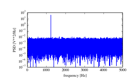
If we average the last half of the spectral density, to exclude the peak, we can recover the noise power on the signal.

>>> np.mean(Pxx_den[256:])
0.0009924865443739191

Now compute and plot the power spectrum.

>>> f, Pxx_spec = signal.periodogram(x, fs, 'flattop', scaling='spectrum')
>>> plt.figure()
>>> plt.semilogy(f, np.sqrt(Pxx_spec))
>>> plt.ylim([1e-4, 1e1])
>>> plt.xlabel('frequency [Hz]')
>>> plt.ylabel('Linear spectrum [V RMS]')
>>> plt.show()

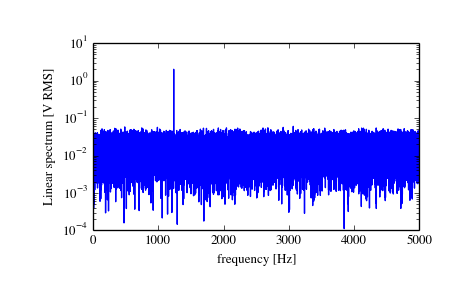
The peak height in the power spectrum is an estimate of the RMS amplitude.

>>> np.sqrt(Pxx_spec.max())
2.0077340678640727