scipy.signal.iirfilter

scipy.signal.iirfilter(N, Wn, rp=None, rs=None, btype='band', analog=False, ftype='butter', output='ba')

IIR digital and analog filter design given order and critical points.

Design an Nth order digital or analog filter and return the filter coefficients in (B,A) (numerator, denominator) or (Z,P,K) form.

Parameters:

N : int

The order of the filter.

Wn : array_like

A scalar or length-2 sequence giving the critical frequencies. For digital filters, Wn is normalized from 0 to 1, where 1 is the Nyquist frequency, pi radians/sample. (Wn is thus in half-cycles / sample.) For analog filters, Wn is an angular frequency (e.g. rad/s).

rp : float, optional

For Chebyshev and elliptic filters, provides the maximum ripple in the passband. (dB)

rs : float, optional

For Chebyshev and elliptic filters, provides the minimum attenuation in the stop band. (dB)

btype : {‘bandpass’, ‘lowpass’, ‘highpass’, ‘bandstop’}, optional

The type of filter. Default is ‘bandpass’.

analog : bool, optional

When True, return an analog filter, otherwise a digital filter is returned.

ftype : str, optional

The type of IIR filter to design:

• Butterworth : ‘butter’
• Chebyshev I : ‘cheby1’
• Chebyshev II : ‘cheby2’
• Cauer/elliptic: ‘ellip’
• Bessel/Thomson: ‘bessel’

output : {‘ba’, ‘zpk’}, optional

Type of output: numerator/denominator (‘ba’) or pole-zero (‘zpk’). Default is ‘ba’.

See also

butter

Filter design using order and critical points

cheby1, cheby2, ellip, bessel

buttord

Find order and critical points from passband and stopband spec

cheb1ord, cheb2ord, ellipord

iirdesign

General filter design using passband and stopband spec

Examples

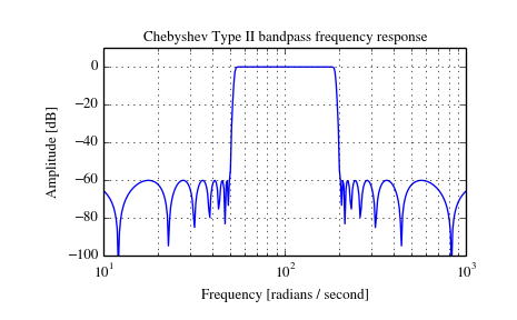
Generate a 17th-order Chebyshev II bandpass filter and plot the frequency response:

>>> from scipy import signal
>>> import matplotlib.pyplot as plt

>>> b, a = signal.iirfilter(17, [50, 200], rs=60, btype='band',
...                         analog=True, ftype='cheby2')
>>> w, h = signal.freqs(b, a, 1000)
>>> fig = plt.figure()
>>> ax = fig.add_subplot(111)
>>> ax.semilogx(w, 20 * np.log10(abs(h)))
>>> ax.set_title('Chebyshev Type II bandpass frequency response')
>>> ax.set_xlabel('Frequency [radians / second]')
>>> ax.set_ylabel('Amplitude [dB]')
>>> ax.axis((10, 1000, -100, 10))
>>> ax.grid(which='both', axis='both')
>>> plt.show()

(Source code)