scipy.stats.f

scipy.stats.f = <scipy.stats._continuous_distns.f_gen object at 0x2b45d2fbb8d0>

An F continuous random variable.

Continuous random variables are defined from a standard form and may require some shape parameters to complete its specification. Any optional keyword parameters can be passed to the methods of the RV object as given below:

Parameters:

x : array_like

quantiles

q : array_like

lower or upper tail probability

dfn, dfd : array_like

shape parameters

loc : array_like, optional

location parameter (default=0)

scale : array_like, optional

scale parameter (default=1)

size : int or tuple of ints, optional

shape of random variates (default computed from input arguments )

moments : str, optional

composed of letters [‘mvsk’] specifying which moments to compute where ‘m’ = mean, ‘v’ = variance, ‘s’ = (Fisher’s) skew and ‘k’ = (Fisher’s) kurtosis. (default=’mv’)

Alternatively, the object may be called (as a function) to fix the shape,

location, and scale parameters returning a “frozen” continuous RV object:

rv = f(dfn, dfd, loc=0, scale=1)

• Frozen RV object with the same methods but holding the given shape, location, and scale fixed.

Notes

The probability density function for f is:

                     df2**(df2/2) * df1**(df1/2) * x**(df1/2-1)
F.pdf(x, df1, df2) = --------------------------------------------
                     (df2+df1*x)**((df1+df2)/2) * B(df1/2, df2/2)

for x > 0.

Examples

>>> from scipy.stats import f
>>> import matplotlib.pyplot as plt
>>> fig, ax = plt.subplots(1, 1)

Calculate a few first moments:

>>> dfn, dfd = 29, 18
>>> mean, var, skew, kurt = f.stats(dfn, dfd, moments='mvsk')

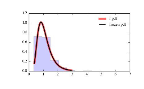
Display the probability density function (pdf):

>>> x = np.linspace(f.ppf(0.01, dfn, dfd),
...               f.ppf(0.99, dfn, dfd), 100)
>>> ax.plot(x, f.pdf(x, dfn, dfd),
...          'r-', lw=5, alpha=0.6, label='f pdf')

Alternatively, freeze the distribution and display the frozen pdf:

>>> rv = f(dfn, dfd)
>>> ax.plot(x, rv.pdf(x), 'k-', lw=2, label='frozen pdf')

Check accuracy of cdf and ppf:

>>> vals = f.ppf([0.001, 0.5, 0.999], dfn, dfd)
>>> np.allclose([0.001, 0.5, 0.999], f.cdf(vals, dfn, dfd))
True

Generate random numbers:

>>> r = f.rvs(dfn, dfd, size=1000)

And compare the histogram:

>>> ax.hist(r, normed=True, histtype='stepfilled', alpha=0.2)
>>> ax.legend(loc='best', frameon=False)
>>> plt.show()

(Source code)

Methods

rvs(dfn, dfd, loc=0, scale=1, size=1)	Random variates.
pdf(x, dfn, dfd, loc=0, scale=1)	Probability density function.
logpdf(x, dfn, dfd, loc=0, scale=1)	Log of the probability density function.
cdf(x, dfn, dfd, loc=0, scale=1)	Cumulative density function.
logcdf(x, dfn, dfd, loc=0, scale=1)	Log of the cumulative density function.
sf(x, dfn, dfd, loc=0, scale=1)	Survival function (1-cdf — sometimes more accurate).
logsf(x, dfn, dfd, loc=0, scale=1)	Log of the survival function.
ppf(q, dfn, dfd, loc=0, scale=1)	Percent point function (inverse of cdf — percentiles).
isf(q, dfn, dfd, loc=0, scale=1)	Inverse survival function (inverse of sf).
moment(n, dfn, dfd, loc=0, scale=1)	Non-central moment of order n
stats(dfn, dfd, loc=0, scale=1, moments=’mv’)	Mean(‘m’), variance(‘v’), skew(‘s’), and/or kurtosis(‘k’).
entropy(dfn, dfd, loc=0, scale=1)	(Differential) entropy of the RV.
fit(data, dfn, dfd, loc=0, scale=1)	Parameter estimates for generic data.
expect(func, dfn, dfd, loc=0, scale=1, lb=None, ub=None, conditional=False, **kwds)	Expected value of a function (of one argument) with respect to the distribution.
median(dfn, dfd, loc=0, scale=1)	Median of the distribution.
mean(dfn, dfd, loc=0, scale=1)	Mean of the distribution.
var(dfn, dfd, loc=0, scale=1)	Variance of the distribution.
std(dfn, dfd, loc=0, scale=1)	Standard deviation of the distribution.
interval(alpha, dfn, dfd, loc=0, scale=1)	Endpoints of the range that contains alpha percent of the distribution