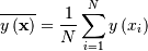
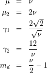
Continuous Statistical Distributions
Overview
All distributions will have location (L) and Scale (S) parameters
along with any shape parameters needed, the names for the shape
parameters will vary. Standard form for the distributions will be
given where  and
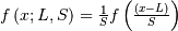
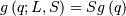
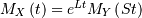
and  The nonstandard forms can be obtained for the various functions using
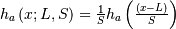
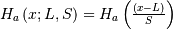
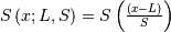
(note
The nonstandard forms can be obtained for the various functions using
(note  is a standard uniform random variate).
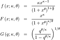
| Function Name | Standard Function | Transformation |
|---|---|---|
| Cumulative Distribution Function (CDF) |  |
 |
| Probability Density Function (PDF) |  |
 |
| Percent Point Function (PPF) | 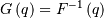 |
 |
| Probability Sparsity Function (PSF) |  |
 |
| Hazard Function (HF) | 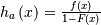 |
 |
| Cumulative Hazard Functon (CHF) |   |
 |
| Survival Function (SF) |  |
 |
| Inverse Survival Function (ISF) |  |
 |
| Moment Generating Function (MGF) | ![M_{Y}\left(t\right)=E\left[e^{Yt}\right]](../../_images/math/633cb572f59446d2f720d80f647eb393aa3a9294.png) |
 |
| Random Variates |  |
 |
| (Differential) Entropy | ![h\left[Y\right]=-\int f\left(y\right)\log f\left(y\right)dy](../../_images/math/152fec670a4351b800367bf33253e1a974fda139.png) |
![h\left[X\right]=h\left[Y\right]+\log S](../../_images/math/74f7333b632c7fcbd636382c65f958f0c37139dc.png) |
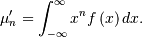
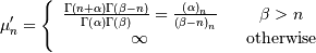
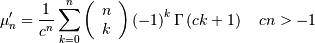
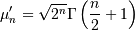
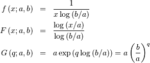
| (Non-central) Moments | ![\mu_{n}^{\prime}=E\left[Y^{n}\right]](../../_images/math/a1b7747dff6611eb46b5314e72b042ac9d42b711.png) |
![E\left[X^{n}\right]=L^{n}\sum_{k=0}^{N}\left(\begin{array}{c} n\\ k\end{array}\right)\left(\frac{S}{L}\right)^{k}\mu_{k}^{\prime}](../../_images/math/e2a343b5608ae448e4ec7f8dcc52167674cfa00a.png) |
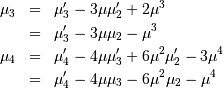
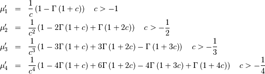
| Central Moments | ![\mu_{n}=E\left[\left(Y-\mu\right)^{n}\right]](../../_images/math/ae9b03a7d7ebeac6657d47066cdb60811f823db2.png) |
![E\left[\left(X-\mu_{X}\right)^{n}\right]=S^{n}\mu_{n}](../../_images/math/8102f1d4323f40b5ed02b6bb183add9ee877a624.png) |
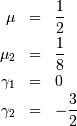
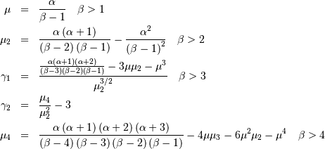
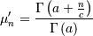
| mean (mode, median), var |  |
 |
| skewness, kurtosis |   |
 |
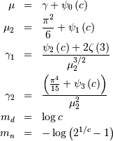
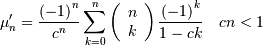
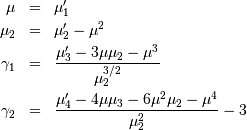
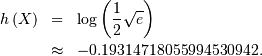
Moments
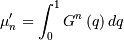
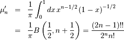
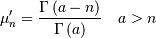
Non-central moments are defined using the PDF
Note, that these can always be computed using the PPF. Substitute  in the above equation and get
which may be easier to compute numerically. Note that  so that
  Central moments are computed similarly
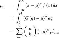
In particular
Skewness is defined as
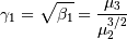
while (Fisher) kurtosis is

so that a normal distribution has a kurtosis of zero.
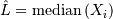
Median and mode
The median,  is defined as the point at which half of the density is on one side
and half on the other. In other words,
is defined as the point at which half of the density is on one side
and half on the other. In other words,  so that

In addition, the mode,  , is defined as the value for which the probability density function
reaches it’s peak
, is defined as the value for which the probability density function
reaches it’s peak
Fitting data
To fit data to a distribution, maximizing the likelihood function is common. Alternatively, some distributions have well-known minimum variance unbiased estimators. These will be chosen by default, but the likelihood function will always be available for minimizing.
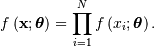
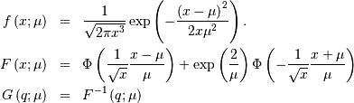
If  is the PDF of a random-variable where
  is a vector of parameters ( e.g.
  and
and  ), then for a collection of
  independent samples from this distribution, the joint distribution the
random vector
independent samples from this distribution, the joint distribution the
random vector  is
is
The maximum likelihood estimate of the parameters are the parameters which maximize this function with fixed and given by the data:
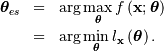
Where
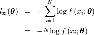
Note that if includes only shape parameters, the location and scale-parameters can
be fit by replacing  with
with  in the log-likelihood function adding
  and minimizing, thus
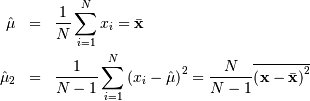
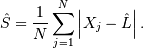
If desired, sample estimates for and (not necessarily maximum likelihood estimates) can be obtained from
samples estimates of the mean and variance using

where  and
and  are assumed known as the mean and variance of the untransformed distribution (when
  and
and  ) and
) and
References
- Documentation for ranlib, rv2, cdflib
- Eric Weisstein~s world of mathematics http://mathworld.wolfram.com/, http://mathworld.wolfram.com/topics/StatisticalDistributions.html
- Documentation to Regress+ by Michael McLaughlin item Engineering and Statistics Handbook (NIST), http://www.itl.nist.gov/div898/handbook/index.htm
- Documentation for DATAPLOT from NIST, http://www.itl.nist.gov/div898/software/dataplot/distribu.htm
- Norman Johnson, Samuel Kotz, and N. Balakrishnan Continuous Univariate Distributions, second edition, Volumes I and II, Wiley & Sons, 1994.
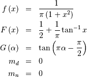
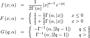
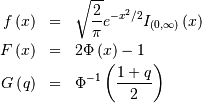
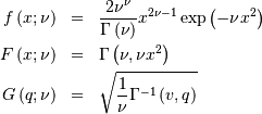
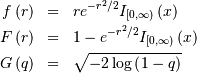
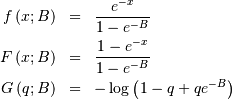
Alpha
One shape parameters  (parameter
  in DATAPLOT
is a scale-parameter). Standard form is
in DATAPLOT
is a scale-parameter). Standard form is 
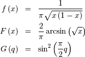
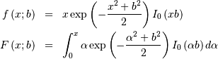
![\begin{eqnarray*} f\left(x;\alpha\right) & = & \frac{1}{x^{2}\Phi\left(\alpha\right)\sqrt{2\pi}}\exp\left(-\frac{1}{2}\left(\alpha-\frac{1}{x}\right)^{2}\right)\\ F\left(x;\alpha\right) & = & \frac{\Phi\left(\alpha-\frac{1}{x}\right)}{\Phi\left(\alpha\right)}\\ G\left(q;\alpha\right) & = & \left[\alpha-\Phi^{-1}\left(q\Phi\left(\alpha\right)\right)\right]^{-1}\end{eqnarray*}](../../_images/math/ef708cb0aeac51b3afc3a3051b612906e014cbfb.png)
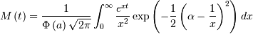
No moments?
![l_{\mathbf{x}}\left(\alpha\right)=N\log\left[\Phi\left(\alpha\right)\sqrt{2\pi}\right]+2N\overline{\log\mathbf{x}}+\frac{N}{2}\alpha^{2}-\alpha\overline{\mathbf{x}^{-1}}+\frac{1}{2}\overline{\mathbf{x}^{-2}}](../../_images/math/9ead47286d5be5dddcf12402f40b5c2d4cdfabaf.png)
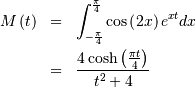
![x\in\left[-\frac{\pi}{4},\frac{\pi}{4}\right]](../../_images/math/da8b9f46752351bf4d22349ae1e09c3078f8abc3.png)
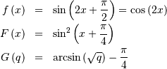
![\begin{eqnarray*} h\left[X\right] & = & 1-\log2\\ & \approx & 0.30685281944005469058\end{eqnarray*}](../../_images/math/85881ff7966a0fab8eed910406a466e9c9d2e6b6.png)
![l_{\mathbf{x}}\left(\cdot\right)=-N\overline{\log\left[\cos\left(2\mathbf{x}\right)\right]}](../../_images/math/5f31071a607c4ed87675d01f1fb040b4d83285ac.png)
 . To get the JKB definition put
  i.e.
i.e.  and
and 
![h\left[X\right]\approx-0.24156447527049044468](../../_images/math/0ab625cd71c421fe77e987b4d7e6fc6212eb1e34.png)

 is also called the Power-function distribution.
![x_{i}\in\left[0,1\right]](../../_images/math/0a4f47f73d1935e0d4833668e1eb5dd5a16bb074.png)
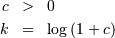
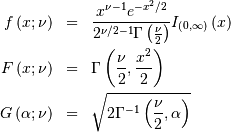
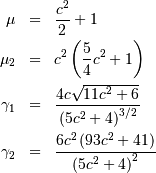
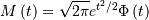
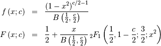
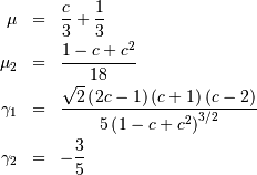
Beta Prime
Defined over 
 (Note the CDF evaluation uses Eq. 3.194.1 on pg. 313 of Gradshteyn &
Ryzhik (sixth edition).
(Note the CDF evaluation uses Eq. 3.194.1 on pg. 313 of Gradshteyn &
Ryzhik (sixth edition).
Therefore,
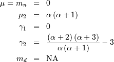
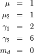
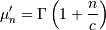
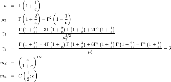
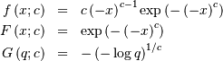
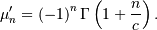
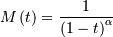
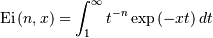
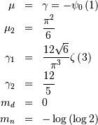
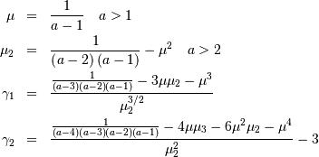
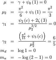
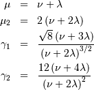
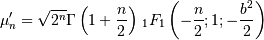
![\begin{eqnarray*} f\left(x;c\right) & = & \frac{c}{k\left(1+cx\right)}I_{\left(0,1\right)}\left(x\right)\\ F\left(x;c\right) & = & \frac{\log\left(1+cx\right)}{k}\\ G\left(\alpha\; c\right) & = & \frac{\left(1+c\right)^{\alpha}-1}{c}\\ M\left(t\right) & = & \frac{1}{k}e^{-t/c}\left[\mathrm{Ei}\left(t+\frac{t}{c}\right)-\mathrm{Ei}\left(\frac{t}{c}\right)\right]\\ \mu & = & \frac{c-k}{ck}\\ \mu_{2} & = & \frac{\left(c+2\right)k-2c}{2ck^{2}}\\ \gamma_{1} & = & \frac{\sqrt{2}\left(12c^{2}-9kc\left(c+2\right)+2k^{2}\left(c\left(c+3\right)+3\right)\right)}{\sqrt{c\left(c\left(k-2\right)+2k\right)}\left(3c\left(k-2\right)+6k\right)}\\ \gamma_{2} & = & \frac{c^{3}\left(k-3\right)\left(k\left(3k-16\right)+24\right)+12kc^{2}\left(k-4\right)\left(k-3\right)+6ck^{2}\left(3k-14\right)+12k^{3}}{3c\left(c\left(k-2\right)+2k\right)^{2}}\\ m_{d} & = & 0\\ m_{n} & = & \sqrt{1+c}-1\end{eqnarray*}](../../_images/math/251884533a42e6634b789cb8d1e254baacbf9d9a.png)
 is the exponential integral function. Also
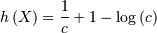
![h\left[X\right]=\frac{1}{2}\log\left(1+c\right)-\log\left(\frac{c}{\log\left(1+c\right)}\right)](../../_images/math/42f707ee161003a8cf65f410e8a60362ebe7ba71.png)
![\begin{eqnarray*} f\left(x;c,d\right) & = & \frac{cd}{x^{c+1}\left(1+x^{-c}\right)^{d+1}}I_{\left(0,\infty\right)}\left(x\right)\\ F\left(x;c,d\right) & = & \left(1+x^{-c}\right)^{-d}\\ G\left(\alpha;c,d\right) & = & \left(\alpha^{-1/d}-1\right)^{-1/c}\\ \mu & = & \frac{\Gamma\left(1-\frac{1}{c}\right)\Gamma\left(\frac{1}{c}+d\right)}{\Gamma\left(d\right)}\\ \mu_{2} & = & \frac{k}{\Gamma^{2}\left(d\right)}\\ \gamma_{1} & = & \frac{1}{\sqrt{k^{3}}}\left[2\Gamma^{3}\left(1-\frac{1}{c}\right)\Gamma^{3}\left(\frac{1}{c}+d\right)+\Gamma^{2}\left(d\right)\Gamma\left(1-\frac{3}{c}\right)\Gamma\left(\frac{3}{c}+d\right)\right.\\ & & \left.-3\Gamma\left(d\right)\Gamma\left(1-\frac{2}{c}\right)\Gamma\left(1-\frac{1}{c}\right)\Gamma\left(\frac{1}{c}+d\right)\Gamma\left(\frac{2}{c}+d\right)\right]\\ \gamma_{2} & = & -3+\frac{1}{k^{2}}\left[6\Gamma\left(d\right)\Gamma\left(1-\frac{2}{c}\right)\Gamma^{2}\left(1-\frac{1}{c}\right)\Gamma^{2}\left(\frac{1}{c}+d\right)\Gamma\left(\frac{2}{c}+d\right)\right.\\ & & -3\Gamma^{4}\left(1-\frac{1}{c}\right)\Gamma^{4}\left(\frac{1}{c}+d\right)+\Gamma^{3}\left(d\right)\Gamma\left(1-\frac{4}{c}\right)\Gamma\left(\frac{4}{c}+d\right)\\ & & \left.-4\Gamma^{2}\left(d\right)\Gamma\left(1-\frac{3}{c}\right)\Gamma\left(1-\frac{1}{c}\right)\Gamma\left(\frac{1}{c}+d\right)\Gamma\left(\frac{3}{c}+d\right)\right]\\ m_{d} & = & \left(\frac{cd-1}{c+1}\right)^{1/c}\,\mathrm{if }cd>1\,\mathrm{otherwise }0\\ m_{n} & = & \left(2^{1/d}-1\right)^{-1/c}\end{eqnarray*}](../../_images/math/22d323ffbc21f3fdb48840fb909ed81303078934.png)
![\begin{eqnarray*} h\left[X\right] & = & \log\left(4\pi\right)\\ & \approx & 2.5310242469692907930.\end{eqnarray*}](../../_images/math/e7e39900c90cc12d561d156325eaad0c94a0df95.png)

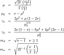
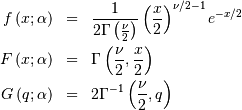
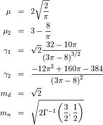
Chi-squared
This is the gamma distribution with and  and
and  where
where  is called the degrees of freedom. If
  are all standard normal distributions, then
  has (standard) chi-square distribution with degrees of freedom.
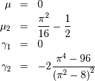
The standard form (most often used in standard form only) is 
![\begin{eqnarray*} f\left(x\right) & = & \frac{1}{2\pi}\left[1+\cos x\right]I_{\left[-\pi,\pi\right]}\left(x\right)\\ F\left(x\right) & = & \frac{1}{2\pi}\left[\pi+x+\sin x\right]I_{\left[-\pi,\pi\right]}\left(x\right)+I_{\left(\pi,\infty\right)}\left(x\right)\\ G\left(\alpha\right) & = & F^{-1}\left(\alpha\right)\\ M\left(t\right) & = & \frac{\sinh\left(\pi t\right)}{\pi t\left(1+t^{2}\right)}\\ \mu=m_{d}=m_{n} & = & 0\\ \mu_{2} & = & \frac{\pi^{2}}{3}-2\\ \gamma_{1} & = & 0\\ \gamma_{2} & = & \frac{-6\left(\pi^{4}-90\right)}{5\left(\pi^{2}-6\right)^{2}}\end{eqnarray*}](../../_images/math/72fd6a314049df8cfbfc6d49a334f19f7a213f69.png)
![\begin{eqnarray*} h\left[X\right] & = & \log\left(4\pi\right)-1\\ & \approx & 1.5310242469692907930.\end{eqnarray*}](../../_images/math/f16cc447c8174eccf67005303aecaf411689b0eb.png)

Doubly Non-central F*
Doubly Non-central t*
Erlang
This is just the Gamma distribution with shape parameter  an integer.
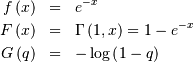
Exponential
This is a special case of the Gamma (and Erlang) distributions with
shape parameter  and the same location and scale parameters. The standard form is
therefore (
and the same location and scale parameters. The standard form is
therefore (  )
)


![h\left[X\right]=1.](../../_images/math/5a8a52fdb10c06d6e2eae836109543c7757d8f1d.png)

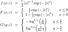
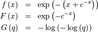
![\begin{eqnarray*} f\left(x;a,c\right) & = & ac\left[1-\exp\left(-x^{c}\right)\right]^{a-1}\exp\left(-x^{c}\right)x^{c-1}\\ F\left(x;a,c\right) & = & \left[1-\exp\left(-x^{c}\right)\right]^{a}\\ G\left(q;a,c\right) & = & \left[-\log\left(1-q^{1/a}\right)\right]^{1/c}\end{eqnarray*}](../../_images/math/067375df988b9e46953783f3979505884636685f.png)
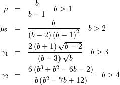
 . Defined for
 ![\begin{eqnarray*} f\left(x;b\right) & = & ebx^{b-1}\exp\left[x^{b}-e^{x^{b}}\right]\\ F\left(x;b\right) & = & 1-\exp\left[1-e^{x^{b}}\right]\\ G\left(q;b\right) & = & \log^{1/b}\left[1-\log\left(1-q\right)\right]\end{eqnarray*}](../../_images/math/90ee36dde65dcda32b0164661bacd280e27cebe7.png)
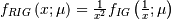
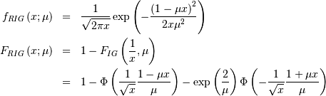
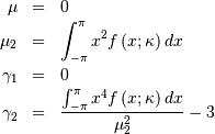
Fatigue Life (Birnbaum-Sanders)
This distribution’s pdf is the average of the inverse-Gaussian  and reciprocal inverse-Gaussian pdf . We follow the notation of JKB here with
  for
for
![\begin{eqnarray*} f\left(x;c\right) & = & \frac{x+1}{2c\sqrt{2\pi x^{3}}}\exp\left(-\frac{\left(x-1\right)^{2}}{2xc^{2}}\right)\\ F\left(x;c\right) & = & \Phi\left(\frac{1}{c}\left(\sqrt{x}-\frac{1}{\sqrt{x}}\right)\right)\\ G\left(q;c\right) & = & \frac{1}{4}\left[c\Phi^{-1}\left(q\right)+\sqrt{c^{2}\left(\Phi^{-1}\left(q\right)\right)^{2}+4}\right]^{2}\end{eqnarray*}](../../_images/math/a12e448600dd3cdb4e4d53a4f55bc55b87777f0e.png)
![M\left(t\right)=c\sqrt{2\pi}\exp\left[\frac{1}{c^{2}}\left(1-\sqrt{1-2c^{2}t}\right)\right]\left(1+\frac{1}{\sqrt{1-2c^{2}t}}\right)](../../_images/math/44910e2ddcdd27655511dc6fb1f9c213fec27b0a.png)

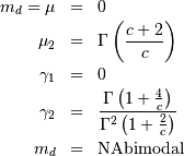
![\begin{eqnarray*} f\left(x;c,d\right) & = & \frac{cx^{c-1}}{\left(1+x^{c}\right)^{2}}I_{\left(0,\infty\right)}\left(x\right)\\ F\left(x;c,d\right) & = & \left(1+x^{-c}\right)^{-1}\\ G\left(\alpha;c,d\right) & = & \left(\alpha^{-1}-1\right)^{-1/c}\\ \mu & = & \Gamma\left(1-\frac{1}{c}\right)\Gamma\left(\frac{1}{c}+1\right)\\ \mu_{2} & = & k\\ \gamma_{1} & = & \frac{1}{\sqrt{k^{3}}}\left[2\Gamma^{3}\left(1-\frac{1}{c}\right)\Gamma^{3}\left(\frac{1}{c}+1\right)+\Gamma\left(1-\frac{3}{c}\right)\Gamma\left(\frac{3}{c}+1\right)\right.\\ & & \left.-3\Gamma\left(1-\frac{2}{c}\right)\Gamma\left(1-\frac{1}{c}\right)\Gamma\left(\frac{1}{c}+1\right)\Gamma\left(\frac{2}{c}+1\right)\right]\\ \gamma_{2} & = & -3+\frac{1}{k^{2}}\left[6\Gamma\left(1-\frac{2}{c}\right)\Gamma^{2}\left(1-\frac{1}{c}\right)\Gamma^{2}\left(\frac{1}{c}+1\right)\Gamma\left(\frac{2}{c}+1\right)\right.\\ & & -3\Gamma^{4}\left(1-\frac{1}{c}\right)\Gamma^{4}\left(\frac{1}{c}+1\right)+\Gamma\left(1-\frac{4}{c}\right)\Gamma\left(\frac{4}{c}+1\right)\\ & & \left.-4\Gamma\left(1-\frac{3}{c}\right)\Gamma\left(1-\frac{1}{c}\right)\Gamma\left(\frac{1}{c}+1\right)\Gamma\left(\frac{3}{c}+1\right)\right]\\ m_{d} & = & \left(\frac{c-1}{c+1}\right)^{1/c}\,\mathrm{if }c>1\,\mathrm{otherwise }0\\ m_{n} & = & 1\end{eqnarray*}](../../_images/math/81f917b534d4f45354dc6acd7dfa620a074ae8d6.png)
![h\left[X\right]=2-\log c.](../../_images/math/6094db396740a9dfc137b1ab872b9891e2761e8f.png)
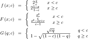
Folded Cauchy
This formula can be expressed in terms of the standard formulas for
the Cauchy distribution (call the cdf  and the pdf
  ). if
). if  is cauchy then
  is folded cauchy. Note that
No moments
Folded Normal
If  is Normal with mean and
  , then
  is a folded normal with shape parameter
  , location parameter
  and scale parameter . This is a special case of the non-central chi distribution with one-
degree of freedom and non-centrality parameter
and scale parameter . This is a special case of the non-central chi distribution with one-
degree of freedom and non-centrality parameter  Note that
  . The standard form of the folded normal is
![M\left(t\right)=\exp\left[\frac{t}{2}\left(t-2c\right)\right]\left(1+e^{2ct}\right)](../../_images/math/ffe0b517c82b4a6f2168ce7df0b21db22fecb943.png)
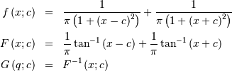
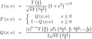
Fratio (or F)
Defined for . The distribution of 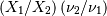 if
if  is chi-squared with
  degrees of freedom and
  is chi-squared with
  degrees of freedom.
![\begin{eqnarray*} f\left(x;\nu_{1},\nu_{2}\right) & = & \frac{\nu_{2}^{\nu_{2}/2}\nu_{1}^{\nu_{1}/2}x^{\nu_{1}/2-1}}{\left(\nu_{2}+\nu_{1}x\right)^{\left(\nu_{1}+\nu_{2}\right)/2}B\left(\frac{\nu_{1}}{2},\frac{\nu_{2}}{2}\right)}\\ F\left(x;v_{1},v_{2}\right) & = & I\left(\frac{\nu_{1}}{2},\frac{\nu_{2}}{2},\frac{\nu_{2}x}{\nu_{2}+\nu_{1}x}\right)\\ G\left(q;\nu_{1},\nu_{2}\right) & = & \left[\frac{\nu_{2}}{I^{-1}\left(\nu_{1}/2,\nu_{2}/2,q\right)}-\frac{\nu_{1}}{\nu_{2}}\right]^{-1}.\end{eqnarray*}](../../_images/math/5aa1757983b2eff0dea69423eec1470095fb7651.png)
![\begin{eqnarray*} \mu & = & \frac{\nu_{2}}{\nu_{2}-2}\quad\nu_{2}>2\\ \mu_{2} & = & \frac{2\nu_{2}^{2}\left(\nu_{1}+\nu_{2}-2\right)}{\nu_{1}\left(\nu_{2}-2\right)^{2}\left(\nu_{2}-4\right)}\quad v_{2}>4\\ \gamma_{1} & = & \frac{2\left(2\nu_{1}+\nu_{2}-2\right)}{\nu_{2}-6}\sqrt{\frac{2\left(\nu_{2}-4\right)}{\nu_{1}\left(\nu_{1}+\nu_{2}-2\right)}}\quad\nu_{2}>6\\ \gamma_{2} & = & \frac{3\left[8+\left(\nu_{2}-6\right)\gamma_{1}^{2}\right]}{2\nu-16}\quad\nu_{2}>8\end{eqnarray*}](../../_images/math/1d320914edaa1b7857884f9a6ccabee016cdf0b1.png)
Fréchet (ExtremeLB, Extreme Value II, Weibull minimum)
A type of extreme-value distribution with a lower bound. Defined for and 
![\begin{eqnarray*} f\left(x;c\right) & = & cx^{c-1}\exp\left(-x^{c}\right)\\ F\left(x;c\right) & = & 1-\exp\left(-x^{c}\right)\\ G\left(q;c\right) & = & \left[-\log\left(1-q\right)\right]^{1/c}\end{eqnarray*}](../../_images/math/16ea329998867c69d645252e4533fca865b6bcc8.png)
![h\left[X\right]=-\frac{\gamma}{c}-\log\left(c\right)+\gamma+1](../../_images/math/09b6c3a2d8f8718a679624e225c53335d5da0056.png)
where  is Euler’s constant and equal to

Fréchet (left-skewed, Extreme Value Type III, Weibull maximum)
Defined for  and .
and .
The mean is the negative of the right-skewed Frechet distribution given above, and the other statistical parameters can be computed from
where is Euler’s constant and equal to
 valid for
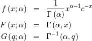
![h\left[X\right]=\Psi\left(a\right)\left[1-a\right]+a+\log\Gamma\left(a\right)](../../_images/math/d007b8c40e205cbc3d182c06c8c998c9158cb29c.png)

Generalized Logistic
Has been used in the analysis of extreme values. Has one shape
parameter  And
And
![\begin{eqnarray*} f\left(x;c\right) & = & \frac{c\exp\left(-x\right)}{\left[1+\exp\left(-x\right)\right]^{c+1}}\\ F\left(x;c\right) & = & \frac{1}{\left[1+\exp\left(-x\right)\right]^{c}}\\ G\left(q;c\right) & = & -\log\left(q^{-1/c}-1\right)\end{eqnarray*}](../../_images/math/0dbccb8d0941231f187ebfbd6afaf23def782b4a.png)
Note that the polygamma function is
where  is a generalization of the Riemann zeta function called the Hurwitz
zeta function Note that
is a generalization of the Riemann zeta function called the Hurwitz
zeta function Note that 
 and defined for
  if
if ![\begin{eqnarray*} f\left(x;c\right) & = & \left(1+cx\right)^{-1-\frac{1}{c}}\\ F\left(x;c\right) & = & 1-\frac{1}{\left(1+cx\right)^{1/c}}\\ G\left(q;c\right) & = & \frac{1}{c}\left[\left(\frac{1}{1-q}\right)^{c}-1\right]\end{eqnarray*}](../../_images/math/f6542b4b89d5c34f62698cdacd3dc726b2758720.png)
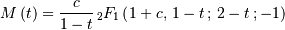
![M\left(t\right)=\left\{ \begin{array}{cc} \left(-\frac{t}{c}\right)^{\frac{1}{c}}e^{-\frac{t}{c}}\left[\Gamma\left(1-\frac{1}{c}\right)+\Gamma\left(-\frac{1}{c},-\frac{t}{c}\right)-\pi\csc\left(\frac{\pi}{c}\right)/\Gamma\left(\frac{1}{c}\right)\right] & c>0\\ \left(\frac{\left|c\right|}{t}\right)^{1/\left|c\right|}\Gamma\left[\frac{1}{\left|c\right|},\frac{t}{\left|c\right|}\right] & c<0\end{array}\right.](../../_images/math/7dc0153ae1706829f09f73cf5ff26ec66aecfdce.png)
![h\left[X\right]=1+c\quad c>0](../../_images/math/7bab714a76093762fcc1482d0df17c9ca6572e13.png)
 and
and 
![\begin{eqnarray*} f\left(x;a,b,c\right) & = & \left(a+b\left(1-e^{-cx}\right)\right)\exp\left[ax-bx+\frac{b}{c}\left(1-e^{-cx}\right)\right]\\ F\left(x;a,b,c\right) & = & 1-\exp\left[ax-bx+\frac{b}{c}\left(1-e^{-cx}\right)\right]\\ G\left(q;a,b,c\right) & = & F^{-1}\end{eqnarray*}](../../_images/math/fa0e37e70be205218dd96be47c6842e0f429025f.png)
Generalized Extreme Value
Extreme value distributions with shape parameter  .
.
For defined on 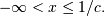
![\begin{eqnarray*} f\left(x;c\right) & = & \exp\left[-\left(1-cx\right)^{1/c}\right]\left(1-cx\right)^{1/c-1}\\ F\left(x;c\right) & = & \exp\left[-\left(1-cx\right)^{1/c}\right]\\ G\left(q;c\right) & = & \frac{1}{c}\left[1-\left(-\log q\right)^{c}\right]\end{eqnarray*}](../../_images/math/252378299611e1f97e3b3c1ecb070451c5913e3c.png)
So,
For  defined on
  For
For  defined over all space
![\begin{eqnarray*} f\left(x;0\right) & = & \exp\left[-e^{-x}\right]e^{-x}\\ F\left(x;0\right) & = & \exp\left[-e^{-x}\right]\\ G\left(q;0\right) & = & -\log\left(-\log q\right)\end{eqnarray*}](../../_images/math/6bfe973580fddd0f29536986733acba131d82365.png)
This is just the (left-skewed) Gumbel distribution for c=0.
Generalized Gamma
A general probability form that reduces to many common distributions:  and
and 
![\begin{eqnarray*} f\left(x;a,c\right) & = & \frac{\left|c\right|x^{ca-1}}{\Gamma\left(a\right)}\exp\left(-x^{c}\right)\\ F\left(x;a,c\right) & = & \begin{array}{cc} \frac{\Gamma\left(a,x^{c}\right)}{\Gamma\left(a\right)} & c>0\\ 1-\frac{\Gamma\left(a,x^{c}\right)}{\Gamma\left(a\right)} & c<0\end{array}\\ G\left(q;a,c\right) & = & \left\{ \Gamma^{-1}\left[a,\Gamma\left(a\right)q\right]\right\} ^{1/c}\quad c>0\\ & & \left\{ \Gamma^{-1}\left[a,\Gamma\left(a\right)\left(1-q\right)\right]\right\} ^{1/c}\quad c<0\end{eqnarray*}](../../_images/math/0312f7dff6300ac2ec5379ce61d5344c8b25d4b9.png)
Special cases are Weibull  , half-normal
 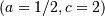 and ordinary gamma distributions
  If
If  then it is the inverted gamma distribution.
![h\left[X\right]=a-a\Psi\left(a\right)+\frac{1}{c}\Psi\left(a\right)+\log\Gamma\left(a\right)-\log\left|c\right|.](../../_images/math/410a7fa43e993a34ca2febff29daa359e642d273.png)
![x\in\left[0,1/c\right]](../../_images/math/97aa4cde127d7371bfc3c34f742dc8fb8729bdb5.png) and
and ![\begin{eqnarray*} f\left(x;c\right) & = & \frac{2\left(1-cx\right)^{\frac{1}{c}-1}}{\left(1+\left(1-cx\right)^{1/c}\right)^{2}}\\ F\left(x;c\right) & = & \frac{1-\left(1-cx\right)^{1/c}}{1+\left(1-cx\right)^{1/c}}\\ G\left(q;c\right) & = & \frac{1}{c}\left[1-\left(\frac{1-q}{1+q}\right)^{c}\right]\end{eqnarray*}](../../_images/math/fcc0e3b804a61ed527bc0c90cdf90369c39963fb.png)
![\begin{eqnarray*} h\left[X\right] & = & 2-\left(2c+1\right)\log2.\end{eqnarray*}](../../_images/math/71ce94ec1c39350c4eb90a52a6b6b67d84d2a0c0.png)
 and
and  (typically also
 ![\begin{eqnarray*} f\left(x;\sigma\right) & = & \frac{1}{x\sqrt{2\pi}}\exp\left[-\frac{1}{2}\left(\log x\right)^{2}\right]\\ F\left(x;\sigma\right) & = & \Phi\left(\log x\right)=\frac{1}{2}\left[1+\mathrm{erf}\left(\frac{\log x}{\sqrt{2}}\right)\right]\\ G\left(q;\sigma\right) & = & \exp\left\{ \Phi^{-1}\left(q\right)\right\} \end{eqnarray*}](../../_images/math/dd4780ec1e7b621f7ab7a48d4bdbc27190a8f489.png)
![\begin{eqnarray*} \mu & = & \sqrt{e}\\ \mu_{2} & = & e\left[e-1\right]\\ \gamma_{1} & = & \sqrt{e-1}\left(2+e\right)\\ \gamma_{2} & = & e^{4}+2e^{3}+3e^{2}-6\end{eqnarray*}](../../_images/math/71829159ae306dbb02086e45437bb7d86050c418.png)
![\begin{eqnarray*} h\left[X\right] & = & \log\left(\sqrt{2\pi e}\right)\\ & \approx & 1.4189385332046727418\end{eqnarray*}](../../_images/math/e4bc890de1e5599c4a0d6d718d9b9c13365877e9.png)
Gompertz (Truncated Gumbel)
For and . In JKB the two shape parameters  are reduced to the single shape-parameter
  . As
. As  is just a scale parameter when
  . If
. If  the distribution reduces to the exponential distribution scaled by
  Thus, the standard form is given as
![\begin{eqnarray*} f\left(x;c\right) & = & ce^{x}\exp\left[-c\left(e^{x}-1\right)\right]\\ F\left(x;c\right) & = & 1-\exp\left[-c\left(e^{x}-1\right)\right]\\ G\left(q;c\right) & = & \log\left[1-\frac{1}{c}\log\left(1-q\right)\right]\end{eqnarray*}](../../_images/math/ed8e92f274ad030b6b37422c18a7e7784854b5ea.png)
![h\left[X\right]=1-\log\left(c\right)-e^{c}\mathrm{Ei}\left(1,c\right),](../../_images/math/4c69a72eb96ce486f5908df55d8619108a8afc1c.png)
where
Gumbel (LogWeibull, Fisher-Tippetts, Type I Extreme Value)
One of a clase of extreme value distributions (right-skewed).
![h\left[X\right]\approx1.0608407169541684911](../../_images/math/e781d67d0db71637b95d99426f249cb18a911a6b.png)
Gumbel Left-skewed (for minimum order statistic)

Note, that is negative the mean for the right-skewed distribution. Similar for
median and mode. All other moments are the same.
![h\left[X\right]\approx1.0608407169541684911.](../../_images/math/a9a7e7053acc36543e998f7972c62c9919a52685.png)
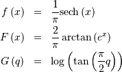
HalfCauchy
If is Hyperbolic Secant distributed then  is Half-Cauchy distributed. Also, if
  is (standard) Cauchy distributed, then
  is Half-Cauchy distributed. Special case of the Folded Cauchy
distribution with
is Half-Cauchy distributed. Special case of the Folded Cauchy
distribution with  The standard form is
![\begin{eqnarray*} f\left(x\right) & = & \frac{2}{\pi\left(1+x^{2}\right)}I_{[0,\infty)}\left(x\right)\\ F\left(x\right) & = & \frac{2}{\pi}\arctan\left(x\right)I_{\left[0,\infty\right]}\left(x\right)\\ G\left(q\right) & = & \tan\left(\frac{\pi}{2}q\right)\end{eqnarray*}](../../_images/math/19f0dd4515c8439696c28ed614dcf2d9b94e12ab.png)
![M\left(t\right)=\cos t+\frac{2}{\pi}\left[\mathrm{Si}\left(t\right)\cos t-\mathrm{Ci}\left(\mathrm{-}t\right)\sin t\right]](../../_images/math/55d3634d5d4aa69362431ca9dc030ca3a55ea39e.png)
No moments, as the integrals diverge.
![\begin{eqnarray*} h\left[X\right] & = & \log\left(2\pi\right)\\ & \approx & 1.8378770664093454836.\end{eqnarray*}](../../_images/math/93b5f371e94a7f6926bdf3740db13dc7f205eead.png)
HalfNormal
This is a special case of the chi distribution with  and
and  and
and  This is also a special case of the folded normal with shape parameter and
  If is (standard) normally distributed then, is half-normal. The standard form is
![\begin{eqnarray*} h\left[X\right] & = & \log\left(\sqrt{\frac{\pi e}{2}}\right)\\ & \approx & 0.72579135264472743239.\end{eqnarray*}](../../_images/math/c7df8dba39140a78f0b7fd73c24e267c2354aea2.png)
Half-Logistic
In the limit as  for the generalized half-logistic we have the half-logistic defined
over Also, the distribution of
for the generalized half-logistic we have the half-logistic defined
over Also, the distribution of  where
where  has logistic distribtution.

![\begin{eqnarray*} h\left[X\right] & = & 2-\log\left(2\right)\\ & \approx & 1.3068528194400546906.\end{eqnarray*}](../../_images/math/491229de309be1729a7209647a5017f9fe37d0da.png)
Hyperbolic Secant
Related to the logistic distribution and used in lifetime analysis.
Standard form is (defined over all  )
)
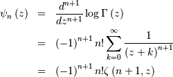
![\begin{eqnarray*} \mu_{n}^{\prime} & = & \frac{1+\left(-1\right)^{n}}{2\pi2^{2n}}n!\left[\zeta\left(n+1,\frac{1}{4}\right)-\zeta\left(n+1,\frac{3}{4}\right)\right]\\ & = & \left\{ \begin{array}{cc} 0 & n\mathrm{ odd}\\ C_{n/2}\frac{\pi^{n}}{2^{n}} & n\mathrm{ even}\end{array}\right.\end{eqnarray*}](../../_images/math/1ce32e0ef787daff47c28f01ac24efa7ff6e93a6.png)
where  is an integer given by
![\begin{eqnarray*} C_{m} & = & \frac{\left(2m\right)!\left[\zeta\left(2m+1,\frac{1}{4}\right)-\zeta\left(2m+1,\frac{3}{4}\right)\right]}{\pi^{2m+1}2^{2m}}\\ & = & 4\left(-1\right)^{m-1}\frac{16^{m}}{2m+1}B_{2m+1}\left(\frac{1}{4}\right)\end{eqnarray*}](../../_images/math/f1a8c23b0dca53c5a9697794d4bf6de9e1fa3454.png)
where  is the Bernoulli polynomial of order
  evaluated at
  Thus
Thus
![h\left[X\right]=\log\left(2\pi\right).](../../_images/math/4f08fe3f0bd2e53bf4cf6b8f8237568dfe59fa67.png)
![x\in\left[0,1\right]](../../_images/math/ede0b6618d567a0e7c9598b5a94ec4590e6a225c.png) ,
, 

![\begin{eqnarray*} f\left(x;a\right) & = & \frac{x^{-a-1}}{\Gamma\left(a\right)}\exp\left(-\frac{1}{x}\right)\\ F\left(x;a\right) & = & \frac{\Gamma\left(a,\frac{1}{x}\right)}{\Gamma\left(a\right)}\\ G\left(q;a\right) & = & \left\{ \Gamma^{-1}\left[a,\Gamma\left(a\right)q\right]\right\} ^{-1}\end{eqnarray*}](../../_images/math/12fc32069dada6768bc8b95fc755af108735db55.png)

![h\left[X\right]=a-\left(a+1\right)\Psi\left(a\right)+\log\Gamma\left(a\right).](../../_images/math/195957a2b5bf18be76f070fc6dd5e14075db28a5.png)
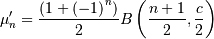
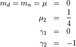
Inverse Normal (Inverse Gaussian)
The standard form involves the shape parameter (in most definitions, is used). (In terms of the regress documentation  ) and
) and  and is not a parameter in that distribution. A standard form is
This is related to the canonical form or JKB “two-parameter “inverse Gaussian when written in it’s full form with scale parameter and location parameter by taking and  then
then  is equal to where is the parameter used by JKB. We prefer this form because of it’s
consistent use of the scale parameter. Notice that in JKB the skew
is equal to where is the parameter used by JKB. We prefer this form because of it’s
consistent use of the scale parameter. Notice that in JKB the skew  and the kurtosis (
  ) are both functions only of
  as shown here, while the variance and mean of the standard form here
are transformed appropriately.
as shown here, while the variance and mean of the standard form here
are transformed appropriately.
![h\left[X\right]=1+\gamma+\frac{\gamma}{c}-\log\left(c\right)](../../_images/math/09a4649a08f6996f32e7fc7f3f05c30b83fa64d4.png)

![\begin{eqnarray*} f\left(x;a,b\right) & = & \frac{b}{x\left(1-x\right)}\phi\left(a+b\log\frac{x}{1-x}\right)\\ F\left(x;a,b\right) & = & \Phi\left(a+b\log\frac{x}{1-x}\right)\\ G\left(q;a,b\right) & = & \frac{1}{1+\exp\left[-\frac{1}{b}\left(\Phi^{-1}\left(q\right)-a\right)\right]}\end{eqnarray*}](../../_images/math/f75dc7a22852c1aab8a1d27ebd25b083d4ec7e7c.png)
 .
.![\begin{eqnarray*} f\left(x;a,b\right) & = & \frac{b}{\sqrt{x^{2}+1}}\phi\left(a+b\log\left(x+\sqrt{x^{2}+1}\right)\right)\\ F\left(x;a,b\right) & = & \Phi\left(a+b\log\left(x+\sqrt{x^{2}+1}\right)\right)\\ G\left(q;a,b\right) & = & \sinh\left[\frac{\Phi^{-1}\left(q\right)-a}{b}\right]\end{eqnarray*}](../../_images/math/ad1bb15ab1e014bd8d8d847551bf10f509076aed.png)
KSone
KStwo
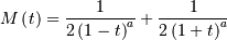
Laplace (Double Exponential, Bilateral Expoooonential)
The ML estimator of the location parameter is
where  is a sequence of mutually independent Laplace RV’s and the median is some number
between the
is a sequence of mutually independent Laplace RV’s and the median is some number
between the  and the
  order statistic ( e.g. take the average of these two) when is even. Also,
Replace  with if it is known. If is known then this estimator is distributed as
  .
.
![\begin{eqnarray*} h\left[X\right] & = & \log\left(2e\right)\\ & \approx & 1.6931471805599453094.\end{eqnarray*}](../../_images/math/3b9054a673f5e40c30b2d7a517baab96a44a2235.png)
Left-skewed Lévy
Special case of Lévy-stable distribution with  and
and  the support is . In standard form
![\begin{eqnarray*} f\left(x\right) & = & \frac{1}{\left|x\right|\sqrt{2\pi\left|x\right|}}\exp\left(-\frac{1}{2\left|x\right|}\right)\\ F\left(x\right) & = & 2\Phi\left(\frac{1}{\sqrt{\left|x\right|}}\right)-1\\ G\left(q\right) & = & -\left[\Phi^{-1}\left(\frac{q+1}{2}\right)\right]^{-2}.\end{eqnarray*}](../../_images/math/b127493a251ea2ebf6c0b009f88bc57bfb1f08dd.png)
No moments.
Lévy
A special case of Lévy-stable distributions with and  . In standard form it is defined for as
![\begin{eqnarray*} f\left(x\right) & = & \frac{1}{x\sqrt{2\pi x}}\exp\left(-\frac{1}{2x}\right)\\ F\left(x\right) & = & 2\left[1-\Phi\left(\frac{1}{\sqrt{x}}\right)\right]\\ G\left(q\right) & = & \left[\Phi^{-1}\left(1-\frac{q}{2}\right)\right]^{-2}.\end{eqnarray*}](../../_images/math/d9097f063e5a5fbd0b329c6dd2649e26a9c10c8a.png)
It has no finite moments.
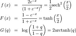
![\begin{eqnarray*} f\left(x\right) & = & \frac{\exp\left(-x\right)}{\left[1+\exp\left(-x\right)\right]^{2}}\\ F\left(x\right) & = & \frac{1}{1+\exp\left(-x\right)}\\ G\left(q\right) & = & -\log\left(1/q-1\right)\end{eqnarray*}](../../_images/math/e6acbc13c4ec6978ffaf7c0a8cb0c4ad89845211.png)
![h\left[X\right]=\log\left(\frac{2e}{c}\right)](../../_images/math/f27016f8adef0134f3da649d6e1c4e0d53520b91.png)
![\begin{eqnarray*} f\left(x;c\right) & = & \frac{\exp\left(cx-e^{x}\right)}{\Gamma\left(c\right)}\\ F\left(x;c\right) & = & \frac{\Gamma\left(c,e^{x}\right)}{\Gamma\left(c\right)}\\ G\left(q;c\right) & = & \log\left[\Gamma^{-1}\left[c,q\Gamma\left(c\right)\right]\right]\end{eqnarray*}](../../_images/math/eb664bf5c717019229e558f3a0086c7ebd3c51a3.png)
![\mu_{n}^{\prime}=\int_{0}^{\infty}\left[\log y\right]^{n}y^{c-1}\exp\left(-y\right)dy.](../../_images/math/339a994bdf6f1adb81914d5171269a3d58a81a10.png)
Log Normal (Cobb-Douglass)
Has one shape parameter  >0. (Notice that the “Regress “
 where is the scale parameter and
  is the mean of the underlying normal distribution). The standard form
is
is the mean of the underlying normal distribution). The standard form
is
![\begin{eqnarray*} f\left(x;\sigma\right) & = & \frac{1}{\sigma x\sqrt{2\pi}}\exp\left[-\frac{1}{2}\left(\frac{\log x}{\sigma}\right)^{2}\right]\\ F\left(x;\sigma\right) & = & \Phi\left(\frac{\log x}{\sigma}\right)\\ G\left(q;\sigma\right) & = & \exp\left\{ \sigma\Phi^{-1}\left(q\right)\right\} \end{eqnarray*}](../../_images/math/5a600331b51896858c67071c356343c33a2ef4ab.png)
![\begin{eqnarray*} \mu & = & \exp\left(\sigma^{2}/2\right)\\ \mu_{2} & = & \exp\left(\sigma^{2}\right)\left[\exp\left(\sigma^{2}\right)-1\right]\\ \gamma_{1} & = & \sqrt{p-1}\left(2+p\right)\\ \gamma_{2} & = & p^{4}+2p^{3}+3p^{2}-6\quad\quad p=e^{\sigma^{2}}\end{eqnarray*}](../../_images/math/943a869c7cddfa0714d8f5647fc63a42b9bdabd6.png)
Notice that using JKB notation we have 
 and we have given the so-called antilognormal form of the
distribution. This is more consistent with the location, scale
parameter description of general probability distributions.
and we have given the so-called antilognormal form of the
distribution. This is more consistent with the location, scale
parameter description of general probability distributions.
![h\left[X\right]=\frac{1}{2}\left[1+\log\left(2\pi\right)+2\log\left(\sigma\right)\right].](../../_images/math/bff51ec964f8209e96a8dea1b9b73d3a75fa2e00.png)
Also, note that if is a log-normally distributed random-variable with and and shape parameter  Then,
Then,  is normally distributed with variance
  and mean

![\begin{eqnarray*} \mu & = & \frac{\Gamma\left(\nu+\frac{1}{2}\right)}{\sqrt{\nu}\Gamma\left(\nu\right)}\\ \mu_{2} & = & \left[1-\mu^{2}\right]\\ \gamma_{1} & = & \frac{\mu\left(1-4v\mu_{2}\right)}{2\nu\mu_{2}^{3/2}}\\ \gamma_{2} & = & \frac{-6\mu^{4}\nu+\left(8\nu-2\right)\mu^{2}-2\nu+1}{\nu\mu_{2}^{2}}\end{eqnarray*}](../../_images/math/5a309de46723228c9ee6082c19f72c02db2b0bf0.png)
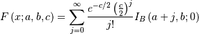
Noncentral chi*
Noncentral chi-squared
The distribution of  where
where  are independent standard normal variables and
  are constants.
  (In communications it is called the Marcum-Q function). Can be thought
of as a Generalized Rayleigh-Rice distribution. For
(In communications it is called the Marcum-Q function). Can be thought
of as a Generalized Rayleigh-Rice distribution. For
![\begin{eqnarray*} f\left(x;\nu,\lambda\right) & = & e^{-\left(\lambda+x\right)/2}\frac{1}{2}\left(\frac{x}{\lambda}\right)^{\left(\nu-2\right)/4}I_{\left(\nu-2\right)/2}\left(\sqrt{\lambda x}\right)\\ F\left(x;\nu,\lambda\right) & = & \sum_{j=0}^{\infty}\left\{ \frac{\left(\lambda/2\right)^{j}}{j!}e^{-\lambda/2}\right\} \mathrm{Pr}\left[\chi_{\nu+2j}^{2}\leq x\right]\\ G\left(q;\nu,\lambda\right) & = & F^{-1}\left(x;\nu,\lambda\right)\end{eqnarray*}](../../_images/math/2f2b33f4e3d91f89ff0ff121d08eeab498de0b69.png)
 and
and 
![\begin{eqnarray*} f\left(x;\lambda,\nu_{1},\nu_{2}\right) & = & \exp\left[\frac{\lambda}{2}+\frac{\left(\lambda\nu_{1}x\right)}{2\left(\nu_{1}x+\nu_{2}\right)}\right]\nu_{1}^{\nu_{1}/2}\nu_{2}^{\nu_{2}/2}x^{\nu_{1}/2-1}\\ & & \times\left(\nu_{2}+\nu_{1}x\right)^{-\left(\nu_{1}+\nu_{2}\right)/2}\frac{\Gamma\left(\frac{\nu_{1}}{2}\right)\Gamma\left(1+\frac{\nu_{2}}{2}\right)L_{\nu_{2}/2}^{\nu_{1}/2-1}\left(-\frac{\lambda\nu_{1}x}{2\left(\nu_{1}x+\nu_{2}\right)}\right)}{B\left(\frac{\nu_{1}}{2},\frac{\nu_{2}}{2}\right)\Gamma\left(\frac{\nu_{1}+\nu_{2}}{2}\right)}\end{eqnarray*}](../../_images/math/1976b7450fa7fca3dc33f32ed2b71e659dcfbbb3.png)
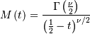
Noncentral t
The distribution of the ratio

where and  are independent and distributed as a standard normal and chi with degrees of freedom. Note
  and
and  .
.
![\begin{eqnarray*} f\left(x;\lambda,\nu\right) & = & \frac{\nu^{\nu/2}\Gamma\left(\nu+1\right)}{2^{\nu}e^{\lambda^{2}/2}\left(\nu+x^{2}\right)^{\nu/2}\Gamma\left(\nu/2\right)}\\ & & \times\left\{ \frac{\sqrt{2}\lambda x\,_{1}F_{1}\left(\frac{\nu}{2}+1;\frac{3}{2};\frac{\lambda^{2}x^{2}}{2\left(\nu+x^{2}\right)}\right)}{\left(\nu+x^{2}\right)\Gamma\left(\frac{\nu+1}{2}\right)}\right.\\ & & -\left.\frac{\,_{1}F_{1}\left(\frac{\nu+1}{2};\frac{1}{2};\frac{\lambda^{2}x^{2}}{2\left(\nu+x^{2}\right)}\right)}{\sqrt{\nu+x^{2}}\Gamma\left(\frac{\nu}{2}+1\right)}\right\} \\ & = & \frac{\Gamma\left(\nu+1\right)}{2^{\left(\nu-1\right)/2}\sqrt{\pi\nu}\Gamma\left(\nu/2\right)}\exp\left[-\frac{\nu\lambda^{2}}{\nu+x^{2}}\right]\\ & & \times\left(\frac{\nu}{\nu+x^{2}}\right)^{\left(\nu-1\right)/2}Hh_{\nu}\left(-\frac{\lambda x}{\sqrt{\nu+x^{2}}}\right)\\ F\left(x;\lambda,\nu\right) & =\end{eqnarray*}](../../_images/math/5b84101fdcf93f6ca9e97371dc44c76305cac979.png)
 and
and 
![h\left[X\right]=\log\left(\sqrt{\frac{2\pi}{e}}\right)+\gamma.](../../_images/math/4fdd4e4e08c58409a4349b34097fd7d945a4b764.png)
Mielke’s Beta-Kappa
A generalized F distribution. Two shape parameters  and
and  , and . The in the DATAPLOT reference is a scale parameter.
 and
and 
 so
so 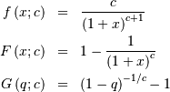
![h\left[X\right]=\frac{1}{c}+1-\log\left(c\right).](../../_images/math/82206004abd97e611150e6362fc1836877abcdee.png)
Power Log Normal
A generalization of the log-normal distribution  and and
![\begin{eqnarray*} f\left(x;\sigma,c\right) & = & \frac{c}{x\sigma}\phi\left(\frac{\log x}{\sigma}\right)\left(\Phi\left(-\frac{\log x}{\sigma}\right)\right)^{c-1}\\ F\left(x;\sigma,c\right) & = & 1-\left(\Phi\left(-\frac{\log x}{\sigma}\right)\right)^{c}\\ G\left(q;\sigma,c\right) & = & \exp\left[-\sigma\Phi^{-1}\left[\left(1-q\right)^{1/c}\right]\right]\end{eqnarray*}](../../_images/math/2c7a857eb26f937c3f07e0d16c5117b68375f504.png)
![\mu_{n}^{\prime}=\int_{0}^{1}\exp\left[-n\sigma\Phi^{-1}\left(y^{1/c}\right)\right]dy](../../_images/math/14b919d259bf5acd7c593c244c5046de114ef559.png)
This distribution reduces to the log-normal distribution when
Power Normal
A generalization of the normal distribution, for
![\begin{eqnarray*} f\left(x;c\right) & = & c\phi\left(x\right)\left(\Phi\left(-x\right)\right)^{c-1}\\ F\left(x;c\right) & = & 1-\left(\Phi\left(-x\right)\right)^{c}\\ G\left(q;c\right) & = & -\Phi^{-1}\left[\left(1-q\right)^{1/c}\right]\end{eqnarray*}](../../_images/math/7e841f3dc819b417c232414286bd788188b16075.png)
![\mu_{n}^{\prime}=\left(-1\right)^{n}\int_{0}^{1}\left[\Phi^{-1}\left(y^{1/c}\right)\right]^{n}dy](../../_images/math/9067527eb19950a3af9c2be2c0d2df69d16cc18f.png)
For  this reduces to the normal distribution.
 : defined for
![h\left[X\right]=1-\frac{1}{a}-\log\left(a\right)](../../_images/math/015df1c5ef54254bf193121619465d60da9f9834.png)
R-distribution
A general-purpose distribution with a variety of shapes controlled by Range of standard distribution is ![x\in\left[-1,1\right]](../../_images/math/aac9c0ae9a862cfe45205524ee5ccc8000faa7ff.png)
The R-distribution with parameter  is the distribution of the correlation coefficient of a random sample
of size drawn from a bivariate normal distribution with
is the distribution of the correlation coefficient of a random sample
of size drawn from a bivariate normal distribution with  The mean of the standard distribution is always zero and as the sample
size grows, the distribution’s mass concentrates more closely about
this mean.
The mean of the standard distribution is always zero and as the sample
size grows, the distribution’s mass concentrates more closely about
this mean.
Rayleigh
This is Chi distribution with and  and
and  (no location parameter is generally used), the mode of the
distribution is
(no location parameter is generally used), the mode of the
distribution is 
![h\left[X\right]=\frac{\gamma}{2}+\log\left(\frac{e}{\sqrt{2}}\right).](../../_images/math/315146081060f755322aa8d4c5cf51258d3fd4a4.png)

![x\in\left[a,b\right]](../../_images/math/11aff69069272c126f4f82f4aae9910257394a76.png)
![\begin{eqnarray*} d & = & \log\left(a/b\right)\\ \mu & = & \frac{a-b}{d}\\ \mu_{2} & = & \mu\frac{a+b}{2}-\mu^{2}=\frac{\left(a-b\right)\left[a\left(d-2\right)+b\left(d+2\right)\right]}{2d^{2}}\\ \gamma_{1} & = & \frac{\sqrt{2}\left[12d\left(a-b\right)^{2}+d^{2}\left(a^{2}\left(2d-9\right)+2abd+b^{2}\left(2d+9\right)\right)\right]}{3d\sqrt{a-b}\left[a\left(d-2\right)+b\left(d+2\right)\right]^{3/2}}\\ \gamma_{2} & = & \frac{-36\left(a-b\right)^{3}+36d\left(a-b\right)^{2}\left(a+b\right)-16d^{2}\left(a^{3}-b^{3}\right)+3d^{3}\left(a^{2}+b^{2}\right)\left(a+b\right)}{3\left(a-b\right)\left[a\left(d-2\right)+b\left(d+2\right)\right]^{2}}-3\\ m_{d} & = & a\\ m_{n} & = & \sqrt{ab}\end{eqnarray*}](../../_images/math/2a18d34c5dfe31509333a99e3e4f89f26c3691bf.png)
![h\left[X\right]=\frac{1}{2}\log\left(ab\right)+\log\left[\log\left(\frac{b}{a}\right)\right].](../../_images/math/b7ae25855eb7bdc59ced849a3614b99e68e5334f.png)
 defined for
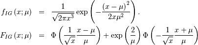
![\begin{eqnarray*} f\left(x\right) & = & \frac{2}{\pi}\sqrt{1-x^{2}}\\ F\left(x\right) & = & \frac{1}{2}+\frac{1}{\pi}\left[x\sqrt{1-x^{2}}+\arcsin x\right]\\ G\left(q\right) & = & F^{-1}\left(q\right)\end{eqnarray*}](../../_images/math/a9008bc02e8f46201e787d6025ef0a79a5fa1fbb.png)
![h\left[X\right]=0.64472988584940017414.](../../_images/math/7e7b4b8a21fe063cf1fe71696460d44ad5e45261.png)
Studentized Range*
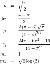
Student t
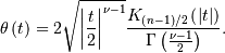
Shape parameter 
 is the incomplete beta integral and
![\begin{eqnarray*} f\left(x;\nu\right) & = & \frac{\Gamma\left(\frac{\nu+1}{2}\right)}{\sqrt{\pi\nu}\Gamma\left(\frac{\nu}{2}\right)\left[1+\frac{x^{2}}{\nu}\right]^{\frac{\nu+1}{2}}}\\ F\left(x;\nu\right) & = & \left\{ \begin{array}{ccc} \frac{1}{2}I\left(\frac{\nu}{2},\frac{1}{2},\frac{\nu}{\nu+x^{2}}\right) & & x\leq0\\ 1-\frac{1}{2}I\left(\frac{\nu}{2},\frac{1}{2},\frac{\nu}{\nu+x^{2}}\right) & & x\geq0\end{array}\right.\\ G\left(q;\nu\right) & = & \left\{ \begin{array}{ccc} -\sqrt{\frac{\nu}{I^{-1}\left(\frac{\nu}{2},\frac{1}{2},2q\right)}-\nu} & & q\leq\frac{1}{2}\\ \sqrt{\frac{\nu}{I^{-1}\left(\frac{\nu}{2},\frac{1}{2},2-2q\right)}-\nu} & & q\geq\frac{1}{2}\end{array}\right.\end{eqnarray*}](../../_images/math/5cb4f75fdfa84acbc3ffb77c121ffd718f0a94bf.png)
As  this distribution approaches the standard normal distribution.
![h\left[X\right]=\frac{1}{4}\log\left(\frac{\pi c\Gamma^{2}\left(\frac{c}{2}\right)}{\Gamma^{2}\left(\frac{c+1}{2}\right)}\right)-\frac{\left(c+1\right)}{4}\left[\Psi\left(\frac{c}{2}\right)-cZ\left(c\right)+\pi\tan\left(\frac{\pi c}{2}\right)+\gamma+2\log2\right]](../../_images/math/047f43a13cbed99d6587ffb4f1490c43b33a98c4.png)
where

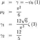
Student Z
The student Z distriubtion is defined over all space with one shape
parameter
Interesting moments are
The moment generating function is
Symmetric Power*
Triangular
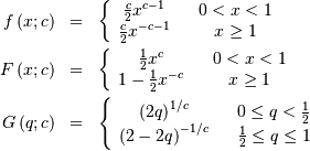
One shape parameter ![c\in[0,1]](../../_images/math/357d86e43515b8c7d9c6921417ae3d4e5d1c6518.png) giving the distance to the peak as a percentage of the total extent of
the non-zero portion. The location parameter is the start of the non-
zero portion, and the scale-parameter is the width of the non-zero
portion. In standard form we have
giving the distance to the peak as a percentage of the total extent of
the non-zero portion. The location parameter is the start of the non-
zero portion, and the scale-parameter is the width of the non-zero
portion. In standard form we have ![x\in\left[0,1\right].](../../_images/math/5f91dd2cc45a717059f916dd5857a1679738460b.png)
Truncated Exponential
This is an exponential distribution defined only over a certain region  . In standard form this is

![h\left[X\right]=\log\left(e^{B}-1\right)+\frac{1+e^{B}\left(B-1\right)}{1-e^{B}}.](../../_images/math/fc900079f64798103ca07cbd6fdf47a37cb8e172.png)
Truncated Normal
A normal distribution restricted to lie within a certain range given
by two parameters and  . Notice that this and correspond to the bounds on in standard form. For
 ![x\in\left[A,B\right]](../../_images/math/322290b5d338f2c17fda326c9203e7409165ce73.png) we get
we get
![\begin{eqnarray*} f\left(x;A,B\right) & = & \frac{\phi\left(x\right)}{\Phi\left(B\right)-\Phi\left(A\right)}\\ F\left(x;A,B\right) & = & \frac{\Phi\left(x\right)-\Phi\left(A\right)}{\Phi\left(B\right)-\Phi\left(A\right)}\\ G\left(q;A,B\right) & = & \Phi^{-1}\left[q\Phi\left(B\right)+\Phi\left(A\right)\left(1-q\right)\right]\end{eqnarray*}](../../_images/math/aae3641756dcc925f89ddbb5c2d1a6c20fab5830.png)
where
![\begin{eqnarray*} f\left(x;\lambda\right) & = & F^{\prime}\left(x;\lambda\right)=\frac{1}{G^{\prime}\left(F\left(x;\lambda\right);\lambda\right)}=\frac{1}{F^{\lambda-1}\left(x;\lambda\right)+\left[1-F\left(x;\lambda\right)\right]^{\lambda-1}}\\ F\left(x;\lambda\right) & = & G^{-1}\left(x;\lambda\right)\\ G\left(p;\lambda\right) & = & \frac{p^{\lambda}-\left(1-p\right)^{\lambda}}{\lambda}\end{eqnarray*}](../../_images/math/55222d78416bedd8404fbc7b3d96e4a730495772.png)


![\begin{eqnarray*} h\left[X\right] & = & \int_{0}^{1}\log\left[G^{\prime}\left(p\right)\right]dp\\ & = & \int_{0}^{1}\log\left[p^{\lambda-1}+\left(1-p\right)^{\lambda-1}\right]dp.\end{eqnarray*}](../../_images/math/4d92321b6da576fd396d3e15c6c897cf4ed2bd32.png)
 In general form, the lower limit is
  the upper limit is

![h\left[X\right]=0](../../_images/math/76762f8440029993aa1ac5eeb47e6235a99007ce.png)
Von Mises
Defined for ![x\in\left[-\pi,\pi\right]](../../_images/math/10579ca7ef9506a45771f4643f6153985efcbdb2.png) with shape parameter
with shape parameter  . Note, the PDF and CDF functions are periodic and are always defined
over regardless of the location parameter. Thus, if an input beyond this
range is given, it is converted to the equivalent angle in this range.
For values of
. Note, the PDF and CDF functions are periodic and are always defined
over regardless of the location parameter. Thus, if an input beyond this
range is given, it is converted to the equivalent angle in this range.
For values of  the PDF and CDF formulas below are used. Otherwise, a normal
approximation with variance
the PDF and CDF formulas below are used. Otherwise, a normal
approximation with variance  is used.
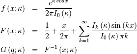
This can be used for defining circular variance.
 . Defined for
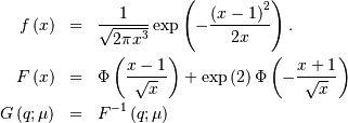
![x\in\left[0,2\pi\right]](../../_images/math/3901855f5dd38d5a7f6ccfffef90fbdd192e6fbc.png)

![\begin{eqnarray*} f\left(x;c\right) & = & \frac{1-c^{2}}{2\pi\left(1+c^{2}-2c\cos x\right)}\\ g_{c}\left(x\right) & = & \frac{1}{\pi}\arctan\left[\frac{1+c}{1-c}\tan\left(\frac{x}{2}\right)\right]\\ r_{c}\left(q\right) & = & 2\arctan\left[\frac{1-c}{1+c}\tan\left(\pi q\right)\right]\\ F\left(x;c\right) & = & \left\{ \begin{array}{ccc} g_{c}\left(x\right) & & 0\leq x<\pi\\ 1-g_{c}\left(2\pi-x\right) & & \pi\leq x\leq2\pi\end{array}\right.\\ G\left(q;c\right) & = & \left\{ \begin{array}{ccc} r_{c}\left(q\right) & & 0\leq q<\frac{1}{2}\\ 2\pi-r_{c}\left(1-q\right) & & \frac{1}{2}\leq q\leq1\end{array}\right.\end{eqnarray*}](../../_images/math/5b0d1fd5bb3418f6fa1dca9d0585ff0116443616.png)
![h\left[X\right]=\log\left(2\pi\left(1-c^{2}\right)\right).](../../_images/math/1fb81345ee749babb79f035400ad252c8d3a24ef.png)