Linear Algebra (scipy.linalg)
When SciPy is built using the optimized ATLAS LAPACK and BLAS libraries, it has very fast linear algebra capabilities. If you dig deep enough, all of the raw lapack and blas libraries are available for your use for even more speed. In this section, some easier-to-use interfaces to these routines are described.
All of these linear algebra routines expect an object that can be converted into a 2-dimensional array. The output of these routines is also a two-dimensional array.
scipy.linalg vs numpy.linalg
scipy.linalg contains all the functions in numpy.linalg. plus some other more advanced ones not contained in numpy.linalg
Another advantage of using scipy.linalg over numpy.linalg is that it is always compiled with BLAS/LAPACK support, while for numpy this is optional. Therefore, the scipy version might be faster depending on how numpy was installed.
Therefore, unless you don’t want to add scipy as a dependency to your numpy program, use scipy.linalg instead of numpy.linalg
numpy.matrix vs 2D numpy.ndarray
The classes that represent matrices, and basic operations such as matrix multiplications and transpose are a part of numpy. For convenience, we summarize the differences between numpy.matrix and numpy.ndarray here.
numpy.matrix is matrix class that has a more convenient interface than numpy.ndarray for matrix operations. This class supports for example MATLAB-like creation syntax via the, has matrix multiplication as default for the * operator, and contains I and T members that serve as shortcuts for inverse and transpose:
>>> import numpy as np
>>> A = np.mat('[1 2;3 4]')
>>> A
matrix([[1, 2],
        [3, 4]])
>>> A.I
matrix([[-2. ,  1. ],
        [ 1.5, -0.5]])
>>> b = np.mat('[5 6]')
>>> b
matrix([[5, 6]])
>>> b.T
matrix([[5],
        [6]])
>>> A*b.T
matrix([[17],
        [39]])
Despite its convenience, the use of the numpy.matrix class is discouraged, since it adds nothing that cannot be accomplished with 2D numpy.ndarray objects, and may lead to a confusion of which class is being used. For example, the above code can be rewritten as:
>>> import numpy as np
>>> from scipy import linalg
>>> A = np.array([[1,2],[3,4]])
>>> A
array([[1, 2],
      [3, 4]])
>>> linalg.inv(A)
array([[-2. ,  1. ],
      [ 1.5, -0.5]])
>>> b = np.array([[5,6]]) #2D array
>>> b
array([[5, 6]])
>>> b.T
array([[5],
      [6]])
>>> A*b #not matrix multiplication!
array([[ 5, 12],
      [15, 24]])
>>> A.dot(b.T) #matrix multiplication
array([[17],
      [39]])
>>> b = np.array([5,6]) #1D array
>>> b
array([5, 6])
>>> b.T  #not matrix transpose!
array([5, 6])
>>> A.dot(b)  #does not matter for multiplication
array([17, 39])
scipy.linalg operations can be applied equally to numpy.matrix or to 2D numpy.ndarray objects.
Basic routines
Finding Inverse
The inverse of a matrix  is the matrix
 such that
  where
where
 is the identity matrix consisting of ones down the
main diagonal. Usually is denoted
is the identity matrix consisting of ones down the
main diagonal. Usually is denoted
 . In SciPy, the matrix inverse of
the Numpy array, A, is obtained using linalg.inv (A) , or
using A.I if A is a Matrix. For example, let
. In SciPy, the matrix inverse of
the Numpy array, A, is obtained using linalg.inv (A) , or
using A.I if A is a Matrix. For example, let
![\[ \mathbf{A=}\left[\begin{array}{ccc} 1 & 3 & 5\\ 2 & 5 & 1\\ 2 & 3 & 8\end{array}\right]\]](../_images/math/f15da1511a57d79b59b079b3b1bd20a88c00cbeb.png)
then
![\[ \mathbf{A^{-1}=\frac{1}{25}\left[\begin{array}{ccc} -37 & 9 & 22\\ 14 & 2 & -9\\ 4 & -3 & 1\end{array}\right]=\left[\begin{array}{ccc} -1.48 & 0.36 & 0.88\\ 0.56 & 0.08 & -0.36\\ 0.16 & -0.12 & 0.04\end{array}\right].}\]](../_images/math/6448dc8dd04285fd3eac2290ee7a0d0d5776b5d9.png)
The following example demonstrates this computation in SciPy
>>> import numpy as np
>>> from scipy import linalg
>>> A = np.array([[1,2],[3,4]])
array([[1, 2],
      [3, 4]])
>>> linalg.inv(A)
array([[-2. ,  1. ],
      [ 1.5, -0.5]])
>>> A.dot(linalg.inv(A)) #double check
array([[  1.00000000e+00,   0.00000000e+00],
      [  4.44089210e-16,   1.00000000e+00]])
Solving linear system
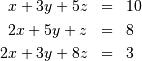
Solving linear systems of equations is straightforward using the scipy command linalg.solve. This command expects an input matrix and a right-hand-side vector. The solution vector is then computed. An option for entering a symmetrix matrix is offered which can speed up the processing when applicable. As an example, suppose it is desired to solve the following simultaneous equations:
We could find the solution vector using a matrix inverse:
![\[ \left[\begin{array}{c} x\\ y\\ z\end{array}\right]=\left[\begin{array}{ccc} 1 & 3 & 5\\ 2 & 5 & 1\\ 2 & 3 & 8\end{array}\right]^{-1}\left[\begin{array}{c} 10\\ 8\\ 3\end{array}\right]=\frac{1}{25}\left[\begin{array}{c} -232\\ 129\\ 19\end{array}\right]=\left[\begin{array}{c} -9.28\\ 5.16\\ 0.76\end{array}\right].\]](../_images/math/10eff05280e41f23e86fae08e79ab0f35ef8e82e.png)
However, it is better to use the linalg.solve command which can be faster and more numerically stable. In this case it however gives the same answer as shown in the following example:
>>> import numpy as np
>>> from scipy import linalg
>>> A = np.array([[1,2],[3,4]])
>>> A
array([[1, 2],
      [3, 4]])
>>> b = np.array([[5],[6]])
>>> b
array([[5],
      [6]])
>>> linalg.inv(A).dot(b) #slow
array([[-4. ],
      [ 4.5]]
>>> A.dot(linalg.inv(A).dot(b))-b #check
array([[  8.88178420e-16],
      [  2.66453526e-15]])
>>> np.linalg.solve(A,b) #fast
array([[-4. ],
      [ 4.5]])
>>> A.dot(np.linalg.solve(A,b))-b #check
array([[ 0.],
      [ 0.]])
Finding Determinant
The determinant of a square matrix is often denoted
 and is a quantity often used in linear
algebra. Suppose
and is a quantity often used in linear
algebra. Suppose  are the elements of the matrix
and let
are the elements of the matrix
and let  be the determinant of the matrix left by removing the
 row and
  column from
. Then for any row
column from
. Then for any row 
![\[ \left|\mathbf{A}\right|=\sum_{j}\left(-1\right)^{i+j}a_{ij}M_{ij}.\]](../_images/math/755bef529c1f89f0d1a25bad420ed878c30d985a.png)
This is a recursive way to define the determinant where the base case
is defined by accepting that the determinant of a  matrix is the only matrix element. In SciPy the determinant can be
calculated with linalg.det . For example, the determinant of
matrix is the only matrix element. In SciPy the determinant can be
calculated with linalg.det . For example, the determinant of
is
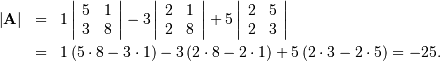
In SciPy this is computed as shown in this example:
>>> import numpy as np
>>> from scipy import linalg
>>> A = np.array([[1,2],[3,4]])
>>> A
array([[1, 2],
      [3, 4]])
>>> linalg.det(A)
-2.0
Computing norms
Matrix and vector norms can also be computed with SciPy. A wide range of norm definitions are available using different parameters to the order argument of linalg.norm . This function takes a rank-1 (vectors) or a rank-2 (matrices) array and an optional order argument (default is 2). Based on these inputs a vector or matrix norm of the requested order is computed.
For vector x , the order parameter can be any real number including inf or -inf. The computed norm is
![\[ \left\Vert \mathbf{x}\right\Vert =\left\{ \begin{array}{cc} \max\left|x_{i}\right| & \textrm{ord}=\textrm{inf}\\ \min\left|x_{i}\right| & \textrm{ord}=-\textrm{inf}\\ \left(\sum_{i}\left|x_{i}\right|^{\textrm{ord}}\right)^{1/\textrm{ord}} & \left|\textrm{ord}\right|<\infty.\end{array}\right.\]](../_images/math/40ce959838b62e756d60da7048ce7b030a6c542b.png)
For matrix the only valid values for norm are 
 inf, and ‘fro’ (or ‘f’) Thus,
![\[ \left\Vert \mathbf{A}\right\Vert =\left\{ \begin{array}{cc} \max_{i}\sum_{j}\left|a_{ij}\right| & \textrm{ord}=\textrm{inf}\\ \min_{i}\sum_{j}\left|a_{ij}\right| & \textrm{ord}=-\textrm{inf}\\ \max_{j}\sum_{i}\left|a_{ij}\right| & \textrm{ord}=1\\ \min_{j}\sum_{i}\left|a_{ij}\right| & \textrm{ord}=-1\\ \max\sigma_{i} & \textrm{ord}=2\\ \min\sigma_{i} & \textrm{ord}=-2\\ \sqrt{\textrm{trace}\left(\mathbf{A}^{H}\mathbf{A}\right)} & \textrm{ord}=\textrm{'fro'}\end{array}\right.\]](../_images/math/554dc8584731014e0bec0140b3fc7b75c00cde7d.png)
where  are the singular values of .
Examples:
>>> import numpy as np
>>> from scipy import linalg
>>> A=np.array([[1,2],[3,4]])
>>> A
array([[1, 2],
      [3, 4]])
>>> linalg.norm(A)
5.4772255750516612
>>> linalg.norm(A,'fro') # frobenius norm is the default
5.4772255750516612
>>> linalg.norm(A,1) # L1 norm (max column sum)
6
>>> linalg.norm(A,-1)
4
>>> linalg.norm(A,inf) # L inf norm (max row sum)
7
Solving linear least-squares problems and pseudo-inverses
Linear least-squares problems occur in many branches of applied
mathematics. In this problem a set of linear scaling coefficients is
sought that allow a model to fit data. In particular it is assumed
that data  is related to data
  through a set of coefficients
  and model functions
 via the model
![\[ y_{i}=\sum_{j}c_{j}f_{j}\left(\mathbf{x}_{i}\right)+\epsilon_{i}\]](../_images/math/824f8f0c8822fb56f2ebf3820efa3027764c70c3.png)
where  represents uncertainty in the data. The
strategy of least squares is to pick the coefficients to
minimize
represents uncertainty in the data. The
strategy of least squares is to pick the coefficients to
minimize
![\[ J\left(\mathbf{c}\right)=\sum_{i}\left|y_{i}-\sum_{j}c_{j}f_{j}\left(x_{i}\right)\right|^{2}.\]](../_images/math/bba7bf382c1b39fb8f7a660d4adc97990b4c83bc.png)
Theoretically, a global minimum will occur when
![\[ \frac{\partial J}{\partial c_{n}^{*}}=0=\sum_{i}\left(y_{i}-\sum_{j}c_{j}f_{j}\left(x_{i}\right)\right)\left(-f_{n}^{*}\left(x_{i}\right)\right)\]](../_images/math/d5e780ba1a0b43644c120d7cdfedf0cd81752b6e.png)
or
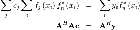
where
![\[ \left\{ \mathbf{A}\right\} _{ij}=f_{j}\left(x_{i}\right).\]](../_images/math/f02400ee00eacc33a25c6f7006209fdfef72102b.png)
When  is invertible, then
![\[ \mathbf{c}=\left(\mathbf{A}^{H}\mathbf{A}\right)^{-1}\mathbf{A}^{H}\mathbf{y}=\mathbf{A}^{\dagger}\mathbf{y}\]](../_images/math/6dc8365db33468ac649416f9b1ee52fb4d3581fa.png)
where  is called the pseudo-inverse of
 Notice that using this definition of
the model can be written
Notice that using this definition of
the model can be written
![\[ \mathbf{y}=\mathbf{Ac}+\boldsymbol{\epsilon}.\]](../_images/math/478f15b1c4b3b59f1a1c04a319df7e48d89575dc.png)
The command linalg.lstsq will solve the linear least squares
problem for  given and
 . In addition linalg.pinv or
linalg.pinv2 (uses a different method based on singular value
decomposition) will find given
. In addition linalg.pinv or
linalg.pinv2 (uses a different method based on singular value
decomposition) will find given
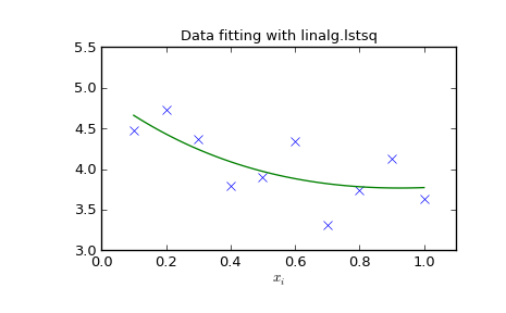
The following example and figure demonstrate the use of linalg.lstsq and linalg.pinv for solving a data-fitting problem. The data shown below were generated using the model:
![\[ y_{i}=c_{1}e^{-x_{i}}+c_{2}x_{i}\]](../_images/math/24ee8d9cd2b039c4556918015d1917b34aa09850.png)
where  for
for  ,
,  ,
and
,
and  Noise is added to and the
coefficients
Noise is added to and the
coefficients  and
and  are estimated using
linear least squares.
are estimated using
linear least squares.
>>> from numpy import *
>>> from scipy import linalg
>>> import matplotlib.pyplot as plt
>>> c1,c2= 5.0,2.0
>>> i = r_[1:11]
>>> xi = 0.1*i
>>> yi = c1*exp(-xi)+c2*xi
>>> zi = yi + 0.05*max(yi)*random.randn(len(yi))
>>> A = c_[exp(-xi)[:,newaxis],xi[:,newaxis]]
>>> c,resid,rank,sigma = linalg.lstsq(A,zi)
>>> xi2 = r_[0.1:1.0:100j]
>>> yi2 = c[0]*exp(-xi2) + c[1]*xi2
>>> plt.plot(xi,zi,'x',xi2,yi2)
>>> plt.axis([0,1.1,3.0,5.5])
>>> plt.xlabel('$x_i$')
>>> plt.title('Data fitting with linalg.lstsq')
>>> plt.show()
Generalized inverse
The generalized inverse is calculated using the command
linalg.pinv or linalg.pinv2. These two commands differ
in how they compute the generalized inverse. The first uses the
linalg.lstsq algorithm while the second uses singular value
decomposition. Let be an  matrix,
then if
matrix,
then if  the generalized inverse is
![\[ \mathbf{A}^{\dagger}=\left(\mathbf{A}^{H}\mathbf{A}\right)^{-1}\mathbf{A}^{H}\]](../_images/math/a437038b602ab343b912b2fc73927ca2fc9627f7.png)
while if  matrix the generalized inverse is
![\[ \mathbf{A}^{\#}=\mathbf{A}^{H}\left(\mathbf{A}\mathbf{A}^{H}\right)^{-1}.\]](../_images/math/f74570d1ea02bded571be7269361aa6de5d7ebad.png)
In both cases for  , then
![\[ \mathbf{A}^{\dagger}=\mathbf{A}^{\#}=\mathbf{A}^{-1}\]](../_images/math/a7ccfa366bb288ff51298fd823f6c9bf7e60825b.png)
as long as is invertible.
Decompositions
In many applications it is useful to decompose a matrix using other representations. There are several decompositions supported by SciPy.
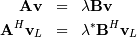
Eigenvalues and eigenvectors
The eigenvalue-eigenvector problem is one of the most commonly
employed linear algebra operations. In one popular form, the
eigenvalue-eigenvector problem is to find for some square matrix
scalars  and corresponding vectors
 such that
![\[ \mathbf{Av}=\lambda\mathbf{v}.\]](../_images/math/1d8e08b5e0feee938bb177c3f90800f6e2f4a7d4.png)
For an  matrix, there are
  (not necessarily
distinct) eigenvalues — roots of the (characteristic) polynomial
(not necessarily
distinct) eigenvalues — roots of the (characteristic) polynomial
![\[ \left|\mathbf{A}-\lambda\mathbf{I}\right|=0.\]](../_images/math/b2662cca5feccf9301f713f3e7c79a985b641cba.png)
The eigenvectors, , are also sometimes called right
eigenvectors to distinguish them from another set of left eigenvectors
that satisfy
![\[ \mathbf{v}_{L}^{H}\mathbf{A}=\lambda\mathbf{v}_{L}^{H}\]](../_images/math/af5d720a35d3b6a2c1ded629d90239b1e25eb9eb.png)
or
![\[ \mathbf{A}^{H}\mathbf{v}_{L}=\lambda^{*}\mathbf{v}_{L}.\]](../_images/math/8774c026418e4bcc15c0fd54ffc01a6303fb3de7.png)
With it’s default optional arguments, the command linalg.eig
returns and  However, it can also
return
However, it can also
return  and just by itself (
linalg.eigvals returns just as well).
and just by itself (
linalg.eigvals returns just as well).
In addtion, linalg.eig can also solve the more general eigenvalue problem
for square matrices and  The
standard eigenvalue problem is an example of the general eigenvalue
problem for
The
standard eigenvalue problem is an example of the general eigenvalue
problem for  When a generalized
eigenvalue problem can be solved, then it provides a decomposition of
as
When a generalized
eigenvalue problem can be solved, then it provides a decomposition of
as
![\[ \mathbf{A}=\mathbf{BV}\boldsymbol{\Lambda}\mathbf{V}^{-1}\]](../_images/math/87276d434b87f1d7912ebdd7c3fc7eafacad3ab6.png)
where  is the collection of eigenvectors into
columns and
is the collection of eigenvectors into
columns and  is a diagonal matrix of
eigenvalues.
is a diagonal matrix of
eigenvalues.
By definition, eigenvectors are only defined up to a constant scale
factor. In SciPy, the scaling factor for the eigenvectors is chosen so
that 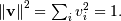
As an example, consider finding the eigenvalues and eigenvectors of the matrix
![\[ \mathbf{A}=\left[\begin{array}{ccc} 1 & 5 & 2\\ 2 & 4 & 1\\ 3 & 6 & 2\end{array}\right].\]](../_images/math/58c752af8057ccb75f3eb73fcf74e012cb8fbbe9.png)
The characteristic polynomial is
![\begin{eqnarray*} \left|\mathbf{A}-\lambda\mathbf{I}\right| & = & \left(1-\lambda\right)\left[\left(4-\lambda\right)\left(2-\lambda\right)-6\right]-\\ & & 5\left[2\left(2-\lambda\right)-3\right]+2\left[12-3\left(4-\lambda\right)\right]\\ & = & -\lambda^{3}+7\lambda^{2}+8\lambda-3.\end{eqnarray*}](../_images/math/67dfe1c28738109b8806fb5d40834ea83eba5352.png)
The roots of this polynomial are the eigenvalues of :
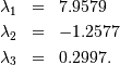
The eigenvectors corresponding to each eigenvalue can be found using the original equation. The eigenvectors associated with these eigenvalues can then be found.
>>> import numpy as np
>>> from scipy import linalg
>>> A = np.array([[1,2],[3,4]])
>>> la,v = linalg.eig(A)
>>> l1,l2 = la
>>> print l1, l2  #eigenvalues
(-0.372281323269+0j) (5.37228132327+0j)
>>> print v[:,0]  #first eigenvector
[-0.82456484  0.56576746]
>>> print v[:,1]  #second eigenvector
[-0.41597356 -0.90937671]
>>> print np.sum(abs(v**2),axis=0) #eigenvectors are unitary
[ 1.  1. ]
>>> v1 = np.array(v[:,0]).T
>>> print linalg.norm(A.dot(v1)-l1*v1) #check the computation
3.23682852457e-16
Singular value decomposition
Singular Value Decompostion (SVD) can be thought of as an extension of
the eigenvalue problem to matrices that are not square. Let
be an matrix with  and
arbitrary. The matrices
and
arbitrary. The matrices  and
and
 are square hermitian matrices [1] of
size and
are square hermitian matrices [1] of
size and  respectively. It is known
that the eigenvalues of square hermitian matrices are real and
non-negative. In addtion, there are at most
respectively. It is known
that the eigenvalues of square hermitian matrices are real and
non-negative. In addtion, there are at most
 identical non-zero eigenvalues of
and
identical non-zero eigenvalues of
and  Define these positive eigenvalues as
  The
square-root of these are called singular values of
The eigenvectors of are collected by
columns into an unitary [2] matrix
while the eigenvectors of
are collected by columns in the
unitary matrix
The
square-root of these are called singular values of
The eigenvectors of are collected by
columns into an unitary [2] matrix
while the eigenvectors of
are collected by columns in the
unitary matrix  , the singular values are collected
in an zero matrix
, the singular values are collected
in an zero matrix
 with main diagonal entries set to
the singular values. Then
with main diagonal entries set to
the singular values. Then
![\[ \mathbf{A=U}\boldsymbol{\Sigma}\mathbf{V}^{H}\]](../_images/math/982143dc39add5009746663baf582d6dc728eafa.png)
is the singular-value decomposition of Every
matrix has a singular value decomposition. Sometimes, the singular
values are called the spectrum of The command
linalg.svd will return ,
 , and as an array of the
singular values. To obtain the matrix
, and as an array of the
singular values. To obtain the matrix  use
linalg.diagsvd. The following example illustrates the use of
linalg.svd .
use
linalg.diagsvd. The following example illustrates the use of
linalg.svd .
>>> import numpy as np
>>> from scipy import linalg
>>> A = np.array([[1,2,3],[4,5,6]])
>>> A
array([[1, 2, 3],
      [4, 5, 6]])
>>> M,N = A.shape
>>> U,s,Vh = linalg.svd(A)
>>> Sig = linalg.diagsvd(s,M,N)
>>> U, Vh = U, Vh
>>> U
array([[-0.3863177 , -0.92236578],
      [-0.92236578,  0.3863177 ]])
>>> Sig
array([[ 9.508032  ,  0.        ,  0.        ],
      [ 0.        ,  0.77286964,  0.        ]])
>>> Vh
array([[-0.42866713, -0.56630692, -0.7039467 ],
      [ 0.80596391,  0.11238241, -0.58119908],
      [ 0.40824829, -0.81649658,  0.40824829]])
>>> U.dot(Sig.dot(Vh)) #check computation
array([[ 1.,  2.,  3.],
      [ 4.,  5.,  6.]])
| [1] | A hermitian matrix  satisfies satisfies  |
| [2] | A unitary matrix satisfies  so that so that  |
LU decomposition
The LU decompostion finds a representation for the matrix as
![\[ \mathbf{A}=\mathbf{PLU}\]](../_images/math/6418ca9f0987baa21818b0df8685344a761b56b1.png)
where  is an permutation matrix (a
permutation of the rows of the identity matrix),
is an permutation matrix (a
permutation of the rows of the identity matrix),  is
in
is
in  lower triangular or trapezoidal matrix (
 ) with unit-diagonal, and
is an upper triangular or trapezoidal matrix. The
SciPy command for this decomposition is linalg.lu .
) with unit-diagonal, and
is an upper triangular or trapezoidal matrix. The
SciPy command for this decomposition is linalg.lu .
Such a decomposition is often useful for solving many simultaneous equations where the left-hand-side does not change but the right hand side does. For example, suppose we are going to solve
![\[ \mathbf{A}\mathbf{x}_{i}=\mathbf{b}_{i}\]](../_images/math/b78d42ead48f836bd05e94dc414deb7186182dfb.png)
for many different  . The LU decomposition allows this to be written as
![\[ \mathbf{PLUx}_{i}=\mathbf{b}_{i}.\]](../_images/math/19939ea9f3ce9b41602abdd5c749a5aaaacf6905.png)
Because is lower-triangular, the equation can be
solved for  and finally
very rapidly using forward- and
back-substitution. An initial time spent factoring
allows for very rapid solution of similar systems of equations in the
future. If the intent for performing LU decomposition is for solving
linear systems then the command linalg.lu_factor should be used
followed by repeated applications of the command
linalg.lu_solve to solve the system for each new
right-hand-side.
and finally
very rapidly using forward- and
back-substitution. An initial time spent factoring
allows for very rapid solution of similar systems of equations in the
future. If the intent for performing LU decomposition is for solving
linear systems then the command linalg.lu_factor should be used
followed by repeated applications of the command
linalg.lu_solve to solve the system for each new
right-hand-side.
Cholesky decomposition
Cholesky decomposition is a special case of LU decomposition
applicable to Hermitian positive definite matrices. When
 and
and
 for all
  ,
then decompositions of can be found so that
,
then decompositions of can be found so that

where is lower-triangular and is
upper triangular. Notice that  The
command linagl.cholesky computes the cholesky
factorization. For using cholesky factorization to solve systems of
equations there are also linalg.cho_factor and
linalg.cho_solve routines that work similarly to their LU
decomposition counterparts.
The
command linagl.cholesky computes the cholesky
factorization. For using cholesky factorization to solve systems of
equations there are also linalg.cho_factor and
linalg.cho_solve routines that work similarly to their LU
decomposition counterparts.
QR decomposition
The QR decomposition (sometimes called a polar decomposition) works
for any array and finds an unitary
matrix  and an upper-trapezoidal
matrix
and an upper-trapezoidal
matrix  such that
![\[ \mathbf{A=QR}.\]](../_images/math/0110430c3f72562038677ae460f41df5b6edd41f.png)
Notice that if the SVD of is known then the QR decomposition can be found
![\[ \mathbf{A}=\mathbf{U}\boldsymbol{\Sigma}\mathbf{V}^{H}=\mathbf{QR}\]](../_images/math/a0e7336badff32ddb382f78f36a93bbae63e3784.png)
implies that  and
and
 Note, however,
that in SciPy independent algorithms are used to find QR and SVD
decompositions. The command for QR decomposition is linalg.qr .
Note, however,
that in SciPy independent algorithms are used to find QR and SVD
decompositions. The command for QR decomposition is linalg.qr .
Schur decomposition
For a square matrix, , the Schur
decomposition finds (not-necessarily unique) matrices
 and
and  such that
![\[ \mathbf{A}=\mathbf{ZT}\mathbf{Z}^{H}\]](../_images/math/63a0676ccac3bd1598fb204e8b85d91d6bc55e50.png)
where is a unitary matrix and is
either upper-triangular or quasi-upper triangular depending on whether
or not a real schur form or complex schur form is requested. For a
real schur form both and are
real-valued when is real-valued. When
is a real-valued matrix the real schur form is only
quasi-upper triangular because  blocks extrude from
the main diagonal corresponding to any complex- valued
eigenvalues. The command linalg.schur finds the Schur
decomposition while the command linalg.rsf2csf converts
and from a real Schur form to a
complex Schur form. The Schur form is especially useful in calculating
functions of matrices.
blocks extrude from
the main diagonal corresponding to any complex- valued
eigenvalues. The command linalg.schur finds the Schur
decomposition while the command linalg.rsf2csf converts
and from a real Schur form to a
complex Schur form. The Schur form is especially useful in calculating
functions of matrices.
The following example illustrates the schur decomposition:
>>> from scipy import linalg
>>> A = mat('[1 3 2; 1 4 5; 2 3 6]')
>>> T,Z = linalg.schur(A)
>>> T1,Z1 = linalg.schur(A,'complex')
>>> T2,Z2 = linalg.rsf2csf(T,Z)
>>> print T
[[ 9.90012467  1.78947961 -0.65498528]
 [ 0.          0.54993766 -1.57754789]
 [ 0.          0.51260928  0.54993766]]
>>> print T2
[[ 9.90012467 +0.00000000e+00j -0.32436598 +1.55463542e+00j
  -0.88619748 +5.69027615e-01j]
 [ 0.00000000 +0.00000000e+00j  0.54993766 +8.99258408e-01j
   1.06493862 +1.37016050e-17j]
 [ 0.00000000 +0.00000000e+00j  0.00000000 +0.00000000e+00j
   0.54993766 -8.99258408e-01j]]
>>> print abs(T1-T2) # different
[[  1.24357637e-14   2.09205364e+00   6.56028192e-01]
 [  0.00000000e+00   4.00296604e-16   1.83223097e+00]
 [  0.00000000e+00   0.00000000e+00   4.57756680e-16]]
>>> print abs(Z1-Z2) # different
[[ 0.06833781  1.10591375  0.23662249]
 [ 0.11857169  0.5585604   0.29617525]
 [ 0.12624999  0.75656818  0.22975038]]
>>> T,Z,T1,Z1,T2,Z2 = map(mat,(T,Z,T1,Z1,T2,Z2))
>>> print abs(A-Z*T*Z.H) # same
[[  1.11022302e-16   4.44089210e-16   4.44089210e-16]
 [  4.44089210e-16   1.33226763e-15   8.88178420e-16]
 [  8.88178420e-16   4.44089210e-16   2.66453526e-15]]
>>> print abs(A-Z1*T1*Z1.H) # same
[[  1.00043248e-15   2.22301403e-15   5.55749485e-15]
 [  2.88899660e-15   8.44927041e-15   9.77322008e-15]
 [  3.11291538e-15   1.15463228e-14   1.15464861e-14]]
>>> print abs(A-Z2*T2*Z2.H) # same
[[  3.34058710e-16   8.88611201e-16   4.18773089e-18]
 [  1.48694940e-16   8.95109973e-16   8.92966151e-16]
 [  1.33228956e-15   1.33582317e-15   3.55373104e-15]]
Interpolative Decomposition
scipy.linalg.interpolative contains routines for computing the
interpolative decomposition (ID) of a matrix. For a matrix  of rank
  this is a factorization

where ![\Pi = [\Pi_{1}, \Pi_{2}]](../_images/math/291cbf4e65281ee63b76ecb97f5fc038df966462.png) is a permutation matrix with
is a permutation matrix with
 , i.e.,
  . This can equivalently be written as
  ,
where
,
where  and
and ![P = [I, T] \Pi^{\mathsf{T}}](../_images/math/aef0bd837b70209742c1c4c3aebc2582a4446856.png) are the skeleton and interpolation matrices, respectively.
are the skeleton and interpolation matrices, respectively.
See also
scipy.linalg.interpolative — for more information.
Matrix Functions
Consider the function  with Taylor series expansion
![\[ f\left(x\right)=\sum_{k=0}^{\infty}\frac{f^{\left(k\right)}\left(0\right)}{k!}x^{k}.\]](../_images/math/adf875f7968f2eacd843a6781a311c30a294d242.png)
A matrix function can be defined using this Taylor series for the
square matrix as
![\[ f\left(\mathbf{A}\right)=\sum_{k=0}^{\infty}\frac{f^{\left(k\right)}\left(0\right)}{k!}\mathbf{A}^{k}.\]](../_images/math/3bb288756a77e30defb3856c78f3f3275944b69d.png)
While, this serves as a useful representation of a matrix function, it is rarely the best way to calculate a matrix function.
Exponential and logarithm functions
The matrix exponential is one of the more common matrix functions. It can be defined for square matrices as
![\[ e^{\mathbf{A}}=\sum_{k=0}^{\infty}\frac{1}{k!}\mathbf{A}^{k}.\]](../_images/math/b90c25a79b0bf9a43a7bb678f6285cdf34c63d0f.png)
The command linalg.expm3 uses this Taylor series definition to compute the matrix exponential. Due to poor convergence properties it is not often used.
Another method to compute the matrix exponential is to find an
eigenvalue decomposition of :
![\[ \mathbf{A}=\mathbf{V}\boldsymbol{\Lambda}\mathbf{V}^{-1}\]](../_images/math/7df93fd626a347846d758355a0a222db1375ee2f.png)
and note that
![\[ e^{\mathbf{A}}=\mathbf{V}e^{\boldsymbol{\Lambda}}\mathbf{V}^{-1}\]](../_images/math/913ee63a8b6d027192a8e0eda61fe6a9cb57c67e.png)
where the matrix exponential of the diagonal matrix is just the exponential of its elements. This method is implemented in linalg.expm2 .
The preferred method for implementing the matrix exponential is to use
scaling and a Padé approximation for  . This algorithm is
implemented as linalg.expm .
. This algorithm is
implemented as linalg.expm .
The inverse of the matrix exponential is the matrix logarithm defined as the inverse of the matrix exponential.
![\[ \mathbf{A}\equiv\exp\left(\log\left(\mathbf{A}\right)\right).\]](../_images/math/32d11c8dcf8b96fa4f2466a53892f850bc713b15.png)
The matrix logarithm can be obtained with linalg.logm .
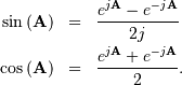
Trigonometric functions
The trigonometric functions  ,
,  , and
, and
 are implemented for matrices in linalg.sinm,
linalg.cosm, and linalg.tanm respectively. The matrix
sin and cosine can be defined using Euler’s identity as
are implemented for matrices in linalg.sinm,
linalg.cosm, and linalg.tanm respectively. The matrix
sin and cosine can be defined using Euler’s identity as
The tangent is
![\[ \tan\left(x\right)=\frac{\sin\left(x\right)}{\cos\left(x\right)}=\left[\cos\left(x\right)\right]^{-1}\sin\left(x\right)\]](../_images/math/430f207b46e2788e19b9cf23f857ab4ac492fe03.png)
and so the matrix tangent is defined as
![\[ \left[\cos\left(\mathbf{A}\right)\right]^{-1}\sin\left(\mathbf{A}\right).\]](../_images/math/3685ed6e1ac7e3a98ea0076b48815f39923f0fe8.png)
Hyperbolic trigonometric functions
The hyperbolic trigonemetric functions  ,
,  ,
and
,
and  can also be defined for matrices using the familiar
definitions:
can also be defined for matrices using the familiar
definitions:
![\begin{eqnarray*} \sinh\left(\mathbf{A}\right) & = & \frac{e^{\mathbf{A}}-e^{-\mathbf{A}}}{2}\\ \cosh\left(\mathbf{A}\right) & = & \frac{e^{\mathbf{A}}+e^{-\mathbf{A}}}{2}\\ \tanh\left(\mathbf{A}\right) & = & \left[\cosh\left(\mathbf{A}\right)\right]^{-1}\sinh\left(\mathbf{A}\right).\end{eqnarray*}](../_images/math/9b414596e47b8daf591e465f76a8bca9bfc3ec26.png)
These matrix functions can be found using linalg.sinhm, linalg.coshm , and linalg.tanhm.
Arbitrary function
Finally, any arbitrary function that takes one complex number and returns a complex number can be called as a matrix function using the command linalg.funm. This command takes the matrix and an arbitrary Python function. It then implements an algorithm from Golub and Van Loan’s book “Matrix Computations “to compute function applied to the matrix using a Schur decomposition. Note that the function needs to accept complex numbers as input in order to work with this algorithm. For example the following code computes the zeroth-order Bessel function applied to a matrix.
>>> from scipy import special, random, linalg
>>> A = random.rand(3,3)
>>> B = linalg.funm(A,lambda x: special.jv(0,x))
>>> print A
[[ 0.72578091  0.34105276  0.79570345]
 [ 0.65767207  0.73855618  0.541453  ]
 [ 0.78397086  0.68043507  0.4837898 ]]
>>> print B
[[ 0.72599893 -0.20545711 -0.22721101]
 [-0.27426769  0.77255139 -0.23422637]
 [-0.27612103 -0.21754832  0.7556849 ]]
>>> print linalg.eigvals(A)
[ 1.91262611+0.j  0.21846476+0.j -0.18296399+0.j]
>>> print special.jv(0, linalg.eigvals(A))
[ 0.27448286+0.j  0.98810383+0.j  0.99164854+0.j]
>>> print linalg.eigvals(B)
[ 0.27448286+0.j  0.98810383+0.j  0.99164854+0.j]
Note how, by virtue of how matrix analytic functions are defined, the Bessel function has acted on the matrix eigenvalues.
Special matrices
SciPy and NumPy provide several functions for creating special matrices that are frequently used in engineering and science.
| Type | Function | Description |
|---|---|---|
| block diagonal | scipy.linalg.block_diag | Create a block diagonal matrix from the provided arrays. |
| circulant | scipy.linalg.circulant | Construct a circulant matrix. |
| companion | scipy.linalg.companion | Create a companion matrix. |
| Hadamard | scipy.linalg.hadamard | Construct a Hadamard matrix. |
| Hankel | scipy.linalg.hankel | Construct a Hankel matrix. |
| Hilbert | scipy.linalg.hilbert | Construct a Hilbert matrix. |
| Inverse Hilbert | scipy.linalg.invhilbert | Construct the inverse of a Hilbert matrix. |
| Leslie | scipy.linalg.leslie | Create a Leslie matrix. |
| Pascal | scipy.linalg.pascal | Create a Pascal matrix. |
| Toeplitz | scipy.linalg.toeplitz | Construct a Toeplitz matrix. |
| Van der Monde | numpy.vander | Generate a Van der Monde matrix. |
For examples of the use of these functions, see their respective docstrings.