numpy.histogram2d

numpy.histogram2d(x, y, bins=10, range=None, normed=False, weights=None)

Compute the bi-dimensional histogram of two data samples.

Parameters :

x : array_like, shape(N,)

A sequence of values to be histogrammed along the first dimension.

y : array_like, shape(M,)

A sequence of values to be histogrammed along the second dimension.

bins : int or [int, int] or array_like or [array, array], optional

The bin specification:

• If int, the number of bins for the two dimensions (nx=ny=bins).
• If [int, int], the number of bins in each dimension (nx, ny = bins).
• If array_like, the bin edges for the two dimensions (x_edges=y_edges=bins).
• If [array, array], the bin edges in each dimension (x_edges, y_edges = bins).

range : array_like, shape(2,2), optional

The leftmost and rightmost edges of the bins along each dimension (if not specified explicitly in the bins parameters): [[xmin, xmax], [ymin, ymax]]. All values outside of this range will be considered outliers and not tallied in the histogram.

normed : bool, optional

If False, returns the number of samples in each bin. If True, returns the bin density, i.e. the bin count divided by the bin area.

weights : array_like, shape(N,), optional

An array of values w_i weighing each sample (x_i, y_i). Weights are normalized to 1 if normed is True. If normed is False, the values of the returned histogram are equal to the sum of the weights belonging to the samples falling into each bin.

Returns :

H : ndarray, shape(nx, ny)

The bi-dimensional histogram of samples x and y. Values in x are histogrammed along the first dimension and values in y are histogrammed along the second dimension.

xedges : ndarray, shape(nx,)

The bin edges along the first dimension.

yedges : ndarray, shape(ny,)

The bin edges along the second dimension.

See also

histogram

1D histogram

histogramdd

Multidimensional histogram

Notes

When normed is True, then the returned histogram is the sample density, defined such that:

where H is the histogram array and the area of bin {i,j}.

Please note that the histogram does not follow the Cartesian convention where x values are on the abcissa and y values on the ordinate axis. Rather, x is histogrammed along the first dimension of the array (vertical), and y along the second dimension of the array (horizontal). This ensures compatibility with histogramdd.

Examples

>>> x, y = np.random.randn(2, 100)
>>> H, xedges, yedges = np.histogram2d(x, y, bins=(5, 8))
>>> H.shape, xedges.shape, yedges.shape
((5, 8), (6,), (9,))

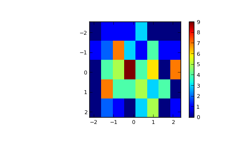
We can now use the Matplotlib to visualize this 2-dimensional histogram:

>>> extent = [yedges[0], yedges[-1], xedges[-1], xedges[0]]
>>> import matplotlib.pyplot as plt
>>> plt.imshow(H, extent=extent, interpolation='nearest')
<matplotlib.image.AxesImage object at ...>
>>> plt.colorbar()
<matplotlib.colorbar.Colorbar instance at ...>
>>> plt.show()

(Source code, png, pdf)