numpy.fft.ifftn
- numpy.fft.ifftn(a, s=None, axes=None)
Compute the N-dimensional inverse discrete Fourier Transform.
This function computes the inverse of the N-dimensional discrete Fourier Transform over any number of axes in an M-dimensional array by means of the Fast Fourier Transform (FFT). In other words, ifftn(fftn(a)) == a to within numerical accuracy. For a description of the definitions and conventions used, see numpy.fft.
The input, analogously to ifft, should be ordered in the same way as is returned by fftn, i.e. it should have the term for zero frequency in all axes in the low-order corner, the positive frequency terms in the first half of all axes, the term for the Nyquist frequency in the middle of all axes and the negative frequency terms in the second half of all axes, in order of decreasingly negative frequency.
Parameters : a : array_like
Input array, can be complex.
s : sequence of ints, optional
Shape (length of each transformed axis) of the output (s[0] refers to axis 0, s[1] to axis 1, etc.). This corresponds to n for ifft(x, n). Along any axis, if the given shape is smaller than that of the input, the input is cropped. If it is larger, the input is padded with zeros. if s is not given, the shape of the input (along the axes specified by axes) is used. See notes for issue on ifft zero padding.
axes : sequence of ints, optional
Axes over which to compute the IFFT. If not given, the last len(s) axes are used, or all axes if s is also not specified. Repeated indices in axes means that the inverse transform over that axis is performed multiple times.
Returns : out : complex ndarray
The truncated or zero-padded input, transformed along the axes indicated by axes, or by a combination of s or a, as explained in the parameters section above.
Raises : ValueError :
If s and axes have different length.
IndexError :
If an element of axes is larger than than the number of axes of a.
See also
- numpy.fft
- Overall view of discrete Fourier transforms, with definitions and conventions used.
- fftn
- The forward n-dimensional FFT, of which ifftn is the inverse.
- ifft
- The one-dimensional inverse FFT.
- ifft2
- The two-dimensional inverse FFT.
- ifftshift
- Undoes fftshift, shifts zero-frequency terms to beginning of array.
Notes
See numpy.fft for definitions and conventions used.
Zero-padding, analogously with ifft, is performed by appending zeros to the input along the specified dimension. Although this is the common approach, it might lead to surprising results. If another form of zero padding is desired, it must be performed before ifftn is called.
Examples
>>> a = np.eye(4)
>>> np.fft.ifftn(np.fft.fftn(a, axes=(0,)), axes=(1,))
array([[ 1.+0.j,  0.+0.j,  0.+0.j,  0.+0.j],
       [ 0.+0.j,  1.+0.j,  0.+0.j,  0.+0.j],
       [ 0.+0.j,  0.+0.j,  1.+0.j,  0.+0.j],
       [ 0.+0.j,  0.+0.j,  0.+0.j,  1.+0.j]])
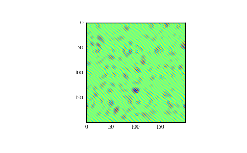
Create and plot an image with band-limited frequency content:
>>> import matplotlib.pyplot as plt
>>> n = np.zeros((200,200), dtype=complex)
>>> n[60:80, 20:40] = np.exp(1j*np.random.uniform(0, 2*np.pi, (20, 20)))
>>> im = np.fft.ifftn(n).real
>>> plt.imshow(im)
<matplotlib.image.AxesImage object at 0x...>
>>> plt.show()
(Source code, png, pdf)

