numpy.meshgrid

numpy.meshgrid(*xi, **kwargs)

Return coordinate matrices from coordinate vectors.

Make N-D coordinate arrays for vectorized evaluations of N-D scalar/vector fields over N-D grids, given one-dimensional coordinate arrays x1, x2,…, xn.

Changed in version 1.9: 1-D and 0-D cases are allowed.

Parameters:

x1, x2,…, xn : array_like

1-D arrays representing the coordinates of a grid.

indexing : {‘xy’, ‘ij’}, optional

Cartesian (‘xy’, default) or matrix (‘ij’) indexing of output. See Notes for more details.

New in version 1.7.0.

sparse : bool, optional

If True a sparse grid is returned in order to conserve memory. Default is False.

New in version 1.7.0.

copy : bool, optional

If False, a view into the original arrays are returned in order to conserve memory. Default is True. Please note that sparse=False, copy=False will likely return non-contiguous arrays. Furthermore, more than one element of a broadcast array may refer to a single memory location. If you need to write to the arrays, make copies first.

New in version 1.7.0.

Returns:

X1, X2,…, XN : ndarray

For vectors x1, x2,…, ‘xn’ with lengths Ni=len(xi) , return (N1, N2, N3,...Nn) shaped arrays if indexing=’ij’ or (N2, N1, N3,...Nn) shaped arrays if indexing=’xy’ with the elements of xi repeated to fill the matrix along the first dimension for x1, the second for x2 and so on.

See also

index_tricks.mgrid

Construct a multi-dimensional “meshgrid” using indexing notation.

index_tricks.ogrid

Construct an open multi-dimensional “meshgrid” using indexing notation.

Notes

This function supports both indexing conventions through the indexing keyword argument. Giving the string ‘ij’ returns a meshgrid with matrix indexing, while ‘xy’ returns a meshgrid with Cartesian indexing. In the 2-D case with inputs of length M and N, the outputs are of shape (N, M) for ‘xy’ indexing and (M, N) for ‘ij’ indexing. In the 3-D case with inputs of length M, N and P, outputs are of shape (N, M, P) for ‘xy’ indexing and (M, N, P) for ‘ij’ indexing. The difference is illustrated by the following code snippet:

xv, yv = np.meshgrid(x, y, sparse=False, indexing='ij')
for i in range(nx):
    for j in range(ny):
        # treat xv[i,j], yv[i,j]

xv, yv = np.meshgrid(x, y, sparse=False, indexing='xy')
for i in range(nx):
    for j in range(ny):
        # treat xv[j,i], yv[j,i]

In the 1-D and 0-D case, the indexing and sparse keywords have no effect.

Examples

>>> nx, ny = (3, 2)
>>> x = np.linspace(0, 1, nx)
>>> y = np.linspace(0, 1, ny)
>>> xv, yv = np.meshgrid(x, y)
>>> xv
array([[0. , 0.5, 1. ],
       [0. , 0.5, 1. ]])
>>> yv
array([[0.,  0.,  0.],
       [1.,  1.,  1.]])
>>> xv, yv = np.meshgrid(x, y, sparse=True)  # make sparse output arrays
>>> xv
array([[0. ,  0.5,  1. ]])
>>> yv
array([[0.],
       [1.]])

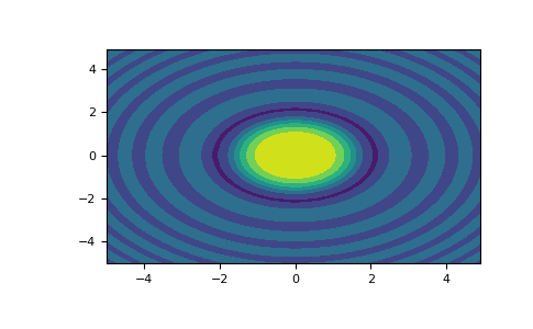
meshgrid is very useful to evaluate functions on a grid.

>>> import matplotlib.pyplot as plt
>>> x = np.arange(-5, 5, 0.1)
>>> y = np.arange(-5, 5, 0.1)
>>> xx, yy = np.meshgrid(x, y, sparse=True)
>>> z = np.sin(xx**2 + yy**2) / (xx**2 + yy**2)
>>> h = plt.contourf(x,y,z)
>>> plt.show()